---
title: "Ic — Task comprehension & Cognitive Reflection (CRT4)"
subtitle: "Descriptive Analyses · GTEMO Experiment"
author: "Eric Guerci"
date: today
format:
html:
theme: flatly
toc: true
toc-depth: 3
toc-title: "Contents"
number-sections: true
code-fold: true
code-summary: "Show code"
code-tools: true
fig-width: 10
fig-height: 6
fig-dpi: 150
smooth-scroll: true
execute:
echo: true
warning: false
message: false
---
```{r setup}
#| include: false
library(tidyverse)
library(gtsummary)
library(gt)
library(ggplot2)
library(patchwork)
library(scales)
library(rstatix)
library(psych)
library(ggridges)
df <- read.csv("../../../data/df_individual_all.csv") |>
mutate(
game_id = factor(game_id, levels = c("BS","MP","PD","SH")),
quiz_perfect = factor(quiz_perfect_q7_9, levels = c(0,1),
labels = c("Errors","Perfect"))
)
col_game <- c("BS" = "#4C72B0", "MP" = "#DD8452",
"PD" = "#55A868", "SH" = "#C44E52")
source("code.R")
```
## Objective
Describe **task comprehension** (quiz errors) and **cognitive reflection ability** (CRT4), and assess whether higher cognitive reflection is associated with better rule comprehension during the experiment.
| Variable | Scale | Description |
|---|---|---|
| `GT_error_q1_to_6` | ≥ 0 | Errors on game-rules quiz (Q1–Q6) |
| `GT_error_q7_8_9` | ≥ 0 | Errors on signal-comprehension quiz (Q7–Q9) |
| `quiz_errors_total` | ≥ 0 | Total cumulative errors across all questions |
| `CRT_totCorrect_corrected` | 0–4 | Correct answers on the CRT4 |
| `CRT_totIntuitive_corrected` | 0–4 | Intuitive (wrong) answers on the CRT4 |
::: callout-note
**CRT4.** This experiment used a 4-item version of the Cognitive Reflection Test (Frederick, 2005). Each item presents a problem with an intuitively compelling but incorrect answer; the correct answer requires overriding the intuitive response through deliberate reasoning. It is not a general IQ test but a specific measure of *reflective* thinking. `CRT_totCorrect_corrected` and `CRT_totIntuitive_corrected` are the corrected variables — **do not use** `CRT_totCorrect` / `CRT_totIntuitive`, which are legacy estimates from a 3-item scoring.
:::
## Data overview
```{r}
#| label: data-overview
df |>
  select(GT_error_q1_to_6, GT_error_q7_8_9, quiz_errors_total,
         CRT_totCorrect_corrected, CRT_totIntuitive_corrected) |>
  skimr::skim()
```
## Descriptive statistics by game
```{r}
#| label: tab-quest
tab_quest
```
::: callout-note
Median (Q1, Q3) for continuous; n (%) for binary. Kruskal-Wallis + η² for continuous; χ² + Cramér's V for categorical. Non-significant differences across games support successful randomisation with respect to cognitive ability and task comprehension.
:::
## Signal comprehension
### Errors by quiz section — violin plots
#### Rules comprehension (Q1–Q6)
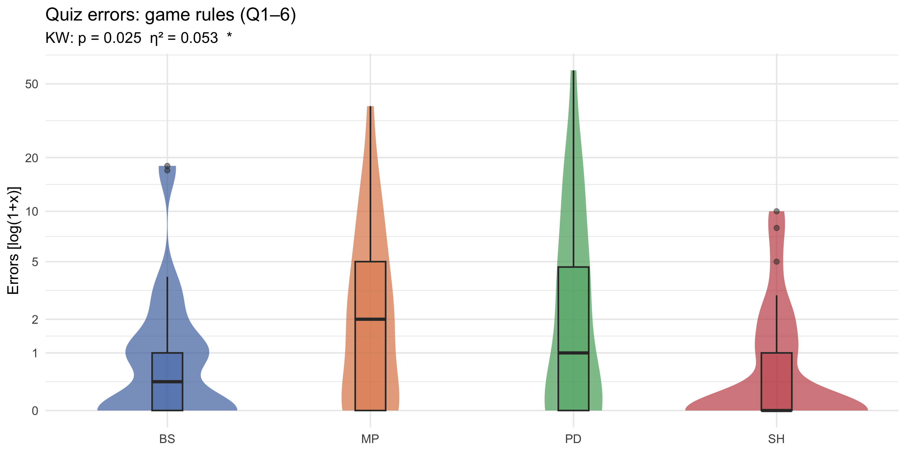
```{r}
#| label: fig-violin-rules
#| fig-cap: "Distribution of errors on game-rules questions (Q1–Q6) by game (log1p y-axis). Violin width shows density; box plot overlay shows quartiles. The log(1+x) transformation compresses the right tail; tick labels show raw error counts."
#| fig-height: 5
p_violin_rules
```
#### Signal comprehension (Q7–Q9)
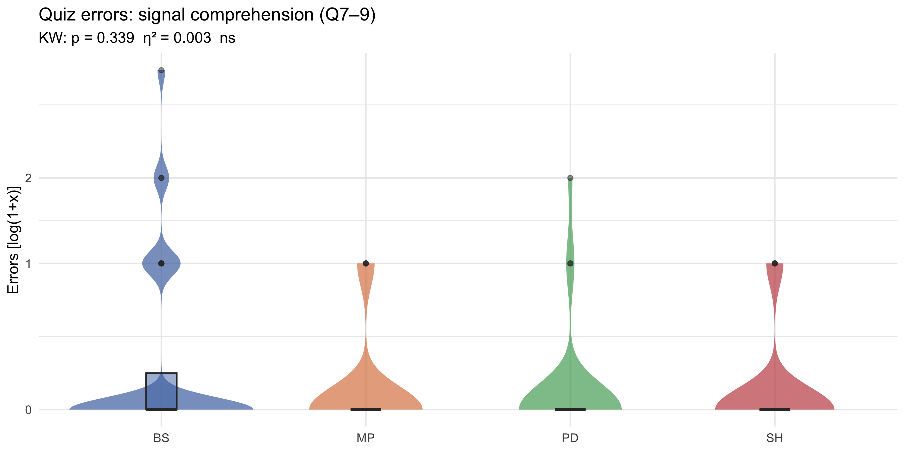
```{r}
#| label: fig-violin-signals
#| fig-cap: "Distribution of errors on signal-comprehension questions (Q7–Q9) by game (log1p y-axis). Violin width shows density; box plot overlay shows quartiles. Tick labels show raw error counts."
#| fig-height: 5
p_violin_signals
```
::: callout-tip
**Comparing the two.** The rules violin (Q1–Q6) and signals violin (Q7–Q9) show different difficulty profiles. If rules errors are concentrated near zero across all games, comprehension of basic mechanics is solid. If signals errors are more dispersed, interpreting signal information during the task is less uniform across participants.
:::
### Total error distribution (ridgeline)
::: callout-note
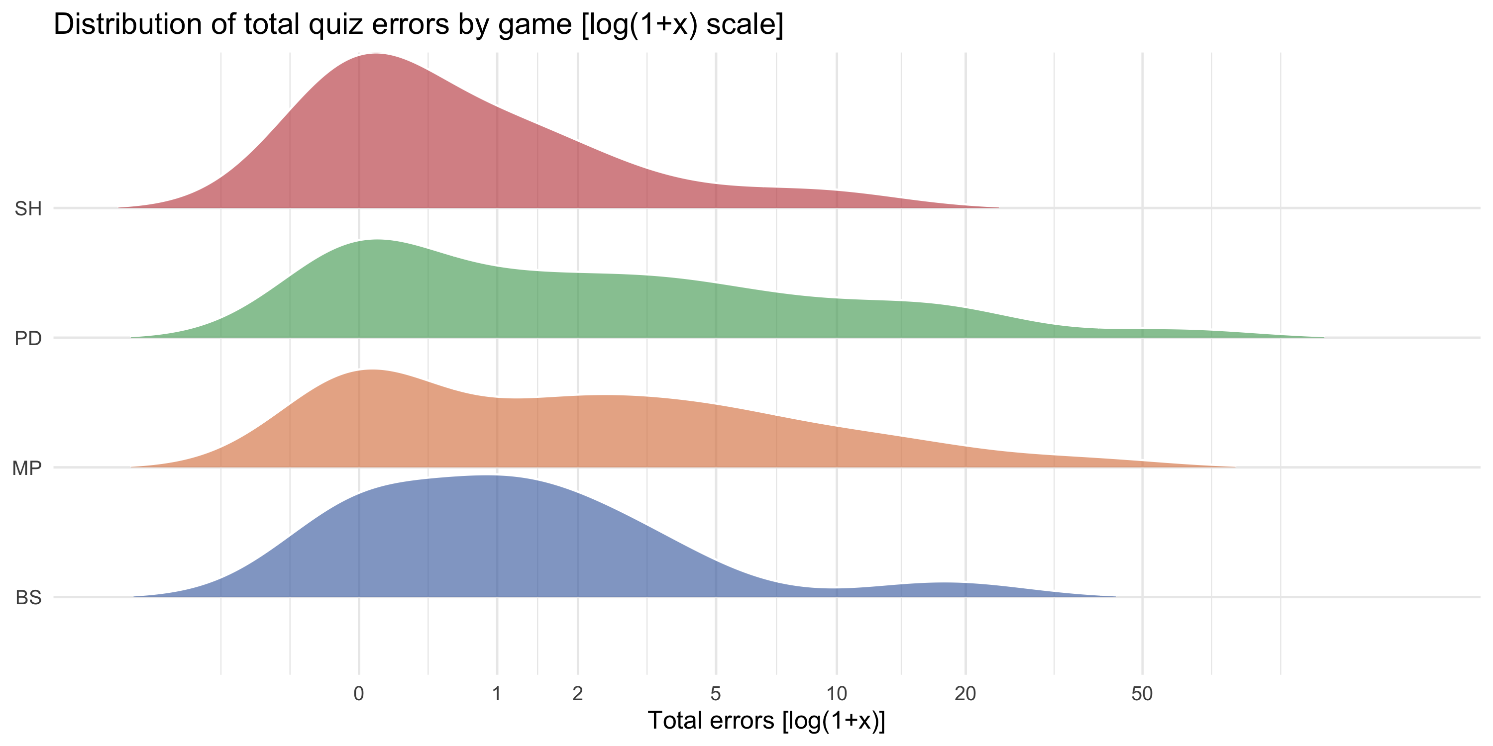
**Log transformation for count data.** Quiz errors are count data (0, 1, 2, ...) with a strong right skew: most participants make few errors, but some make many. The `log(1+x)` transformation (`log1p`) is applied throughout: it compresses the right tail, maps zero exactly to zero (no offset needed), and is consistent with all other error plots in this section. Tick labels always show raw error counts.
:::
```{r}
#| label: fig-ridgeline
#| fig-cap: "Ridgeline density of total quiz errors by game [log(1+x) scale]. Tick labels show raw error counts. Strong right skew is typical: most participants made few errors, with a long tail in every condition."
#| fig-height: 5
p_ridgeline
```
## CRT4 performance
### Distribution by game
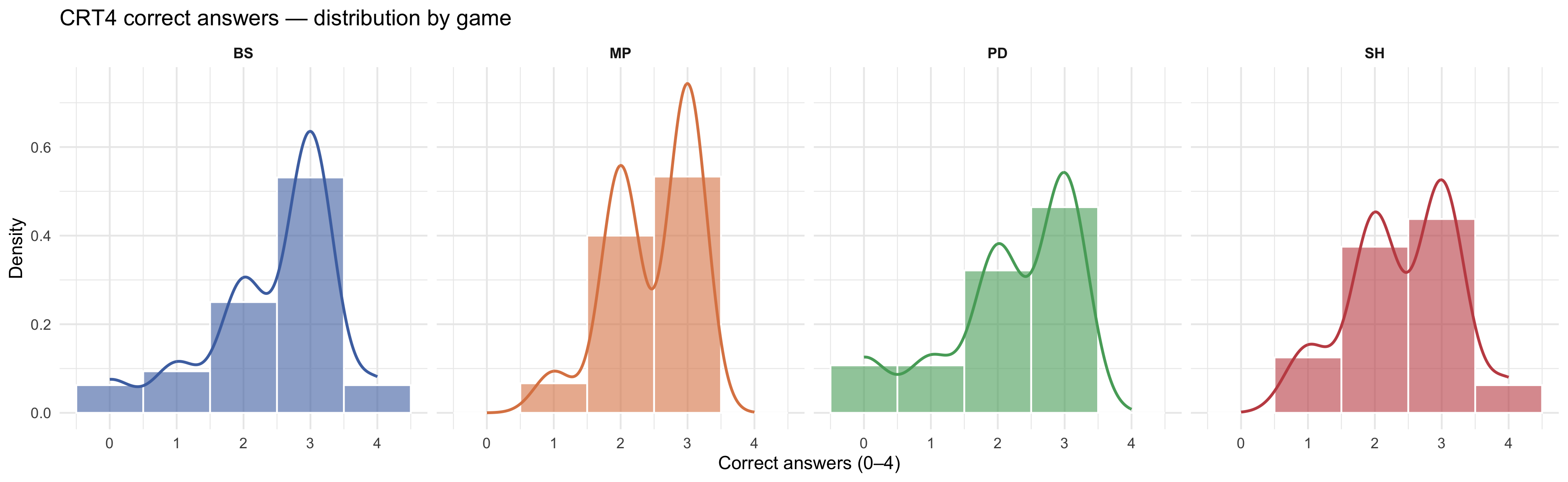
```{r}
#| label: fig-crt-hist
#| fig-cap: "Distribution of CRT4 correct answers (0–4) by game. Histogram with overlaid kernel density. Scores range 0–4 (4-item version)."
#| fig-width: 13
#| fig-height: 4
p_crt_hist
```
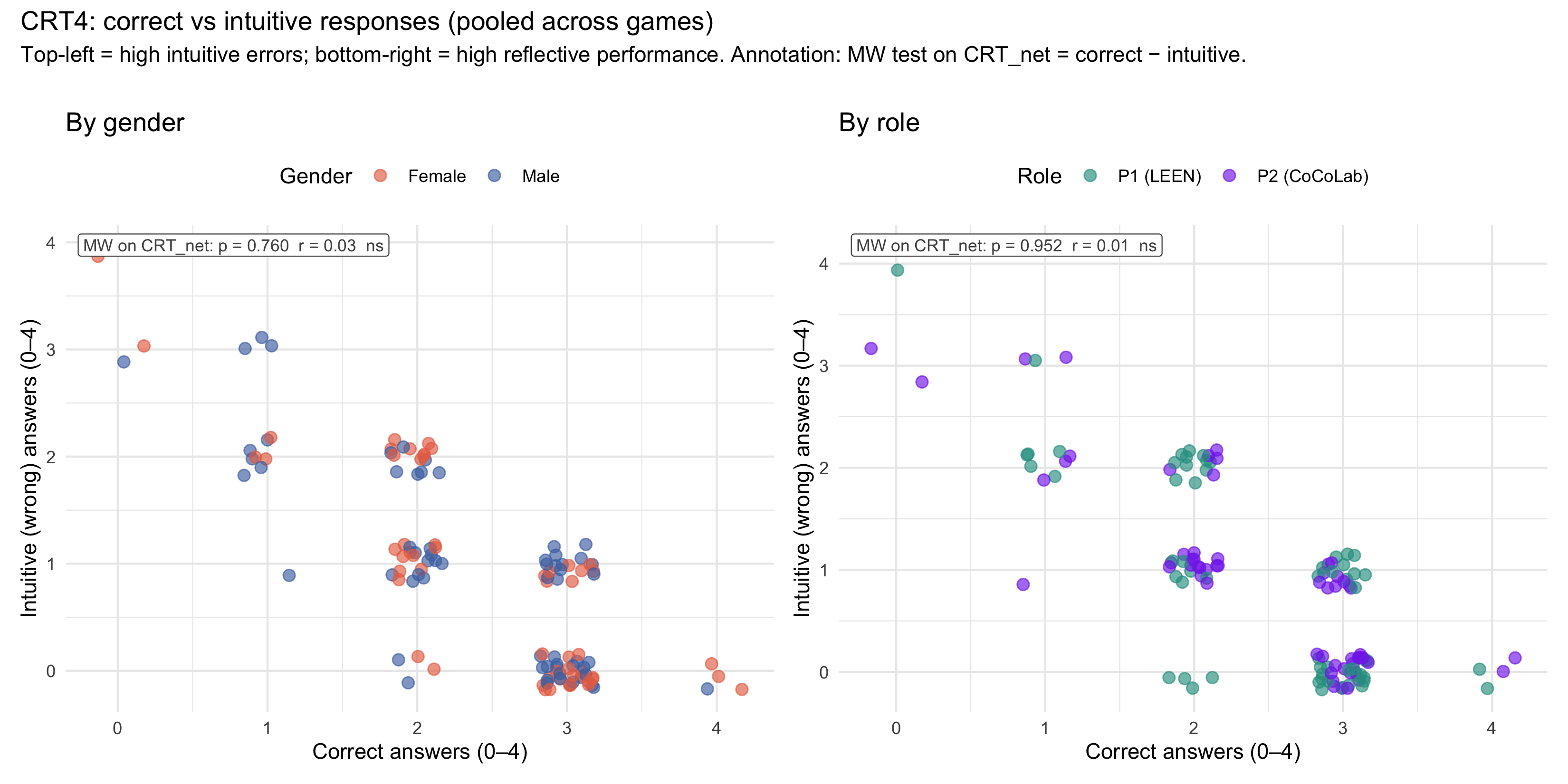
### Correct vs intuitive responses
::: callout-note
**Statistical test.** Because both variables are discrete (0–4) with a built-in constraint (correct + intuitive ≤ 4), a linear regression interaction would be biased by the bounded scale. Instead, we summarise each participant's reflective performance with a single **net CRT score** (CRT~net~ = correct − intuitive, range −4 to +4) and compare groups with a **Mann-Whitney U test** (reported in the annotation). As a robustness check, a **binomial GLM with interaction** (`correct/4 ~ intuitive × group`, family = Binomial) tests whether the correct~intuitive slope differs by group; results are reported below.
:::
```{r}
#| label: fig-crt-scatter
#| fig-cap: "CRT4 correct vs intuitive answers, pooled across game conditions. Left: by gender; right: by role. Annotation: Mann-Whitney U test on CRT~net~ (= correct − intuitive). Bottom-right = high reflective performance; top-left = predominantly intuitive."
#| fig-width: 11
#| fig-height: 5.5
p_crt_scatter
```
```{r}
#| label: tab-binom-interaction
#| tbl-cap: "Binomial GLM robustness check: interaction term testing whether the correct ~ intuitive slope differs by group. A non-significant interaction (ns) means the negative correct–intuitive relationship is equally strong in both groups."
gt_binom_interaction
```
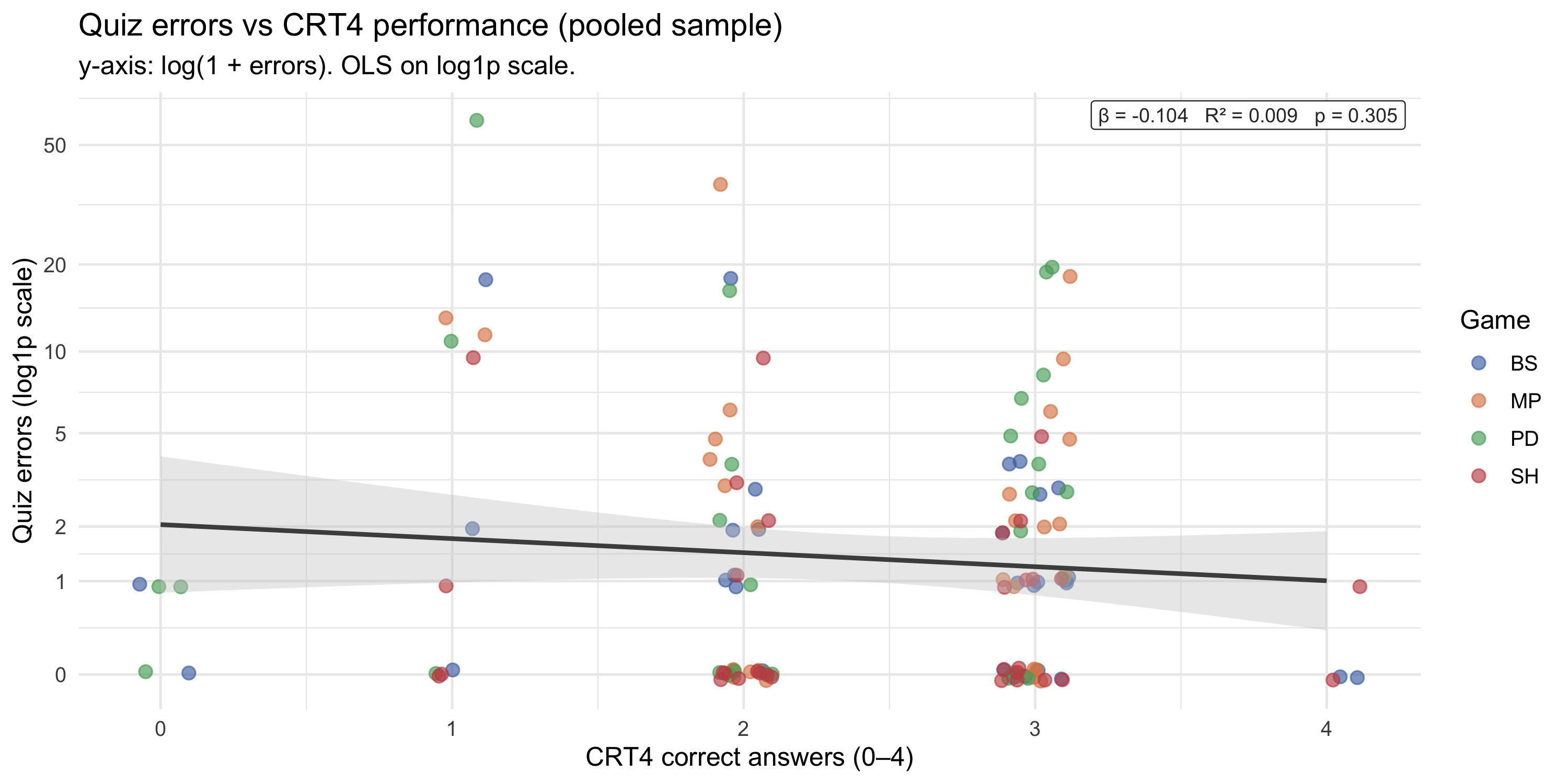
## CRT4 vs quiz comprehension
Does higher cognitive reflection predict fewer comprehension errors?
```{r}
#| label: fig-quiz-vs-crt
#| fig-cap: "Total quiz errors [log(1+x) scale] against CRT4 correct answers. OLS line fitted on the log1p-transformed outcome; top-right label reports β, R², and p-value. Tick labels show raw error counts. Points coloured by game."
#| fig-height: 5
p_quiz_vs_crt
```
```{r}
#| label: crt-quiz-corr
cor_res <- cor.test(df$CRT_totCorrect_corrected, df$quiz_errors_total,
                    method = "spearman", exact = FALSE)

tibble(
  Test      = "Spearman \u03c1",
  Statistic = round(cor_res$statistic, 2),
  rho       = round(cor_res$estimate, 3),
  p_value   = signif(cor_res$p.value, 3)
) |>
  gt() |>
  tab_header(title = "Correlation: CRT4 correct answers vs total quiz errors") |>
  tab_style(style = cell_text(weight = "bold"),
            locations = cells_column_labels())
```
::: callout-note
A negative ρ indicates that participants who scored higher on the CRT4 tended to make fewer quiz errors — consistent with cognitive reflection ability supporting better comprehension of complex experimental instructions.
:::
## CRT time vs cognitive reflection: non-linear analysis
On the CRT, longer deliberation time is theoretically associated with successful override of intuitive errors. However, this relationship may be **non-monotonic**: while moderate reflection time helps participants override intuitive (wrong) answers, participants who spend *very long* times may be those who struggle with the task — extra time reflects difficulty rather than productive deliberation. We investigate this hypothesis progressively: linear baseline → non-parametric smooth → quadratic test → segmented regression with estimated breakpoint.
::: callout-note
**Note on quiz timing.** Quiz completion times (GT_time_quiz_total_sec) contain negative values due to clock drift in the oTree data collection and have been excluded from analysis. CRT response times are clean and retained.
:::
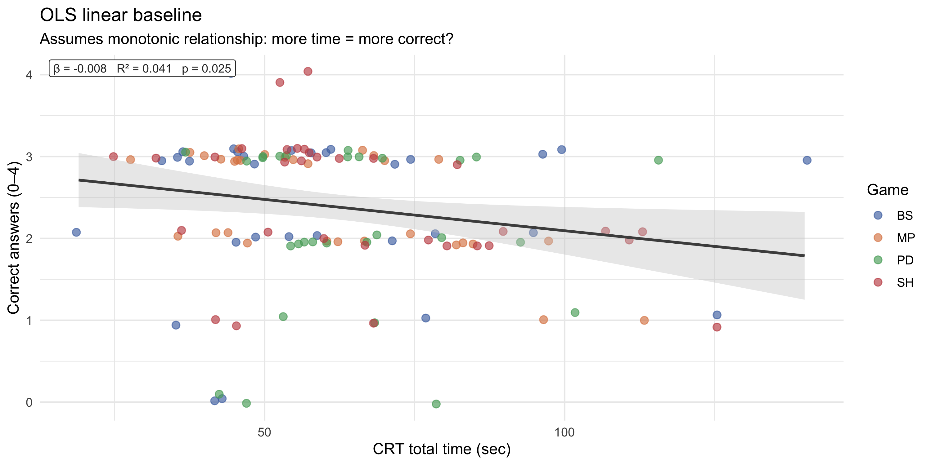
### OLS linear baseline
```{r}
#| label: fig-crt-ols
#| fig-cap: "OLS linear fit: CRT4 time vs correct answers. A positive slope suggests that more time = more correct answers on average, but this model assumes monotonicity."
#| fig-height: 5
p_crt_ols
```
The linear model provides the simplest summary: does spending more time on the CRT predict better performance? However, it imposes a constant marginal effect of time across the entire range and cannot capture the hypothesised threshold.
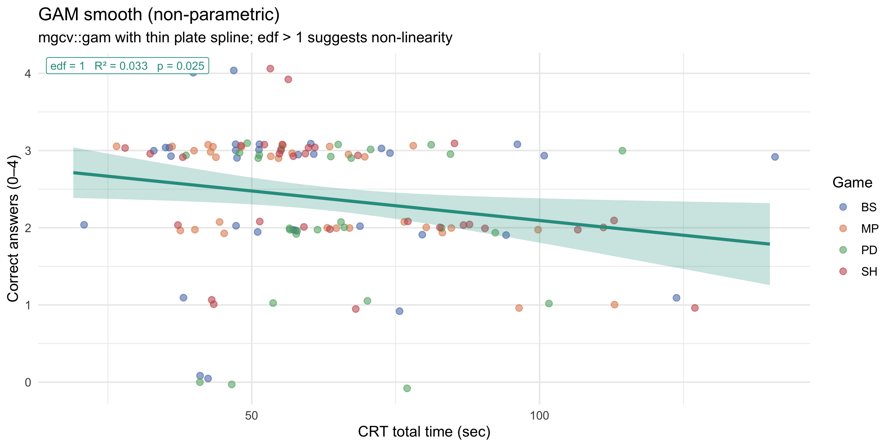
### GAM smooth — visual evidence of non-linearity
```{r}
#| label: fig-crt-gam
#| fig-cap: "GAM non-parametric smooth (mgcv, thin plate spline). If the effective degrees of freedom (edf) exceed 1, the data suggest a non-linear relationship. The 95% confidence band shows uncertainty in the smooth."
#| fig-height: 5
p_crt_gam
```
::: callout-tip
**Reading the GAM.** The effective degrees of freedom (edf) reported in the annotation quantify the *wiggliness* of the smooth. edf ≈ 1 means the relationship is essentially linear; edf > 1 indicates curvature. If the smooth clearly bends — rising then flattening or dropping — this motivates a parametric model with a turning point.
:::
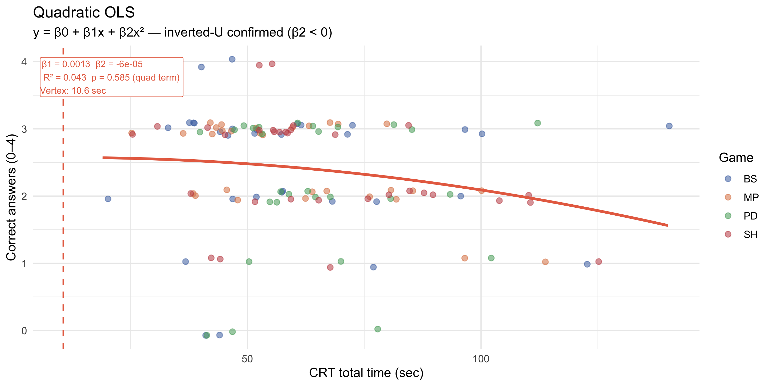
### Quadratic OLS — parametric test of concavity
```{r}
#| label: fig-crt-quad
#| fig-cap: "Quadratic OLS: y = β₀ + β₁·time + β₂·time². A significant negative β₂ confirms an inverted-U shape. The dashed vertical line marks the vertex (estimated turning point)."
#| fig-height: 5
p_crt_quad
```
The quadratic model adds a single parameter (β₂) to test for concavity. A significant negative β₂ confirms the inverted-U hypothesis. The vertex of the parabola provides a *symmetric* estimate of the turning point — but symmetry is a strong assumption that the segmented model relaxes.
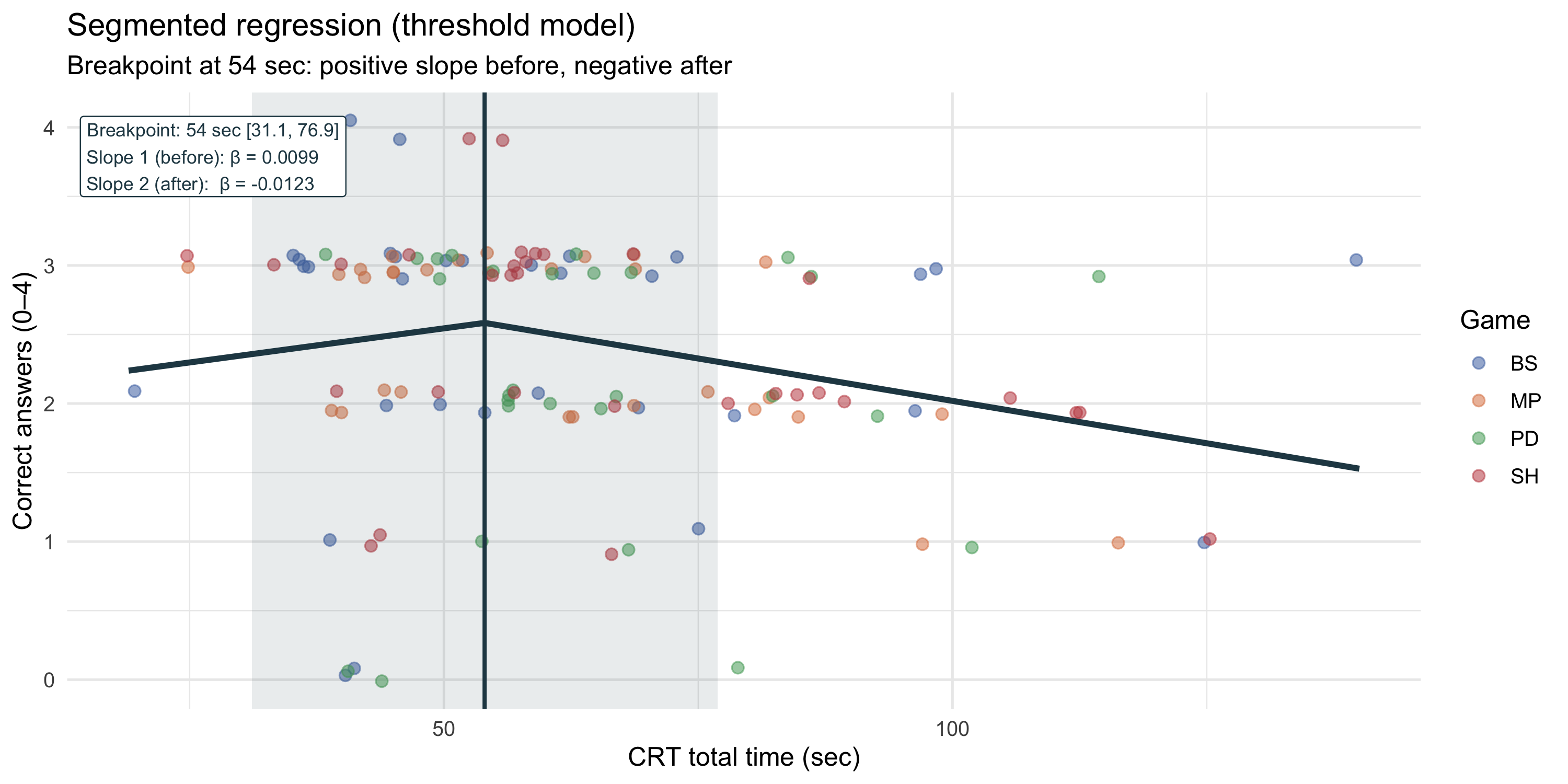
### Segmented regression — threshold estimation
```{r}
#| label: fig-crt-seg
#| fig-cap: "Segmented (piecewise) regression with endogenously estimated breakpoint. The vertical line marks the estimated threshold; shaded band shows the 95% CI. Slopes before and after the breakpoint are estimated independently."
#| fig-height: 5
p_crt_seg
```
::: callout-important
**Segmented regression** (Muggeo, 2003) estimates the breakpoint ψ endogenously and fits two separate linear slopes — one before and one after ψ. Unlike the quadratic model, it does not impose symmetry around the turning point. This makes it the most appropriate model if the mechanism differs qualitatively on either side of the threshold: *productive reflection* (slope 1) vs *struggling without learning* (slope 2).
:::
### Model comparison
```{r}
#| label: tab-model-comp
tab_model_comp
```
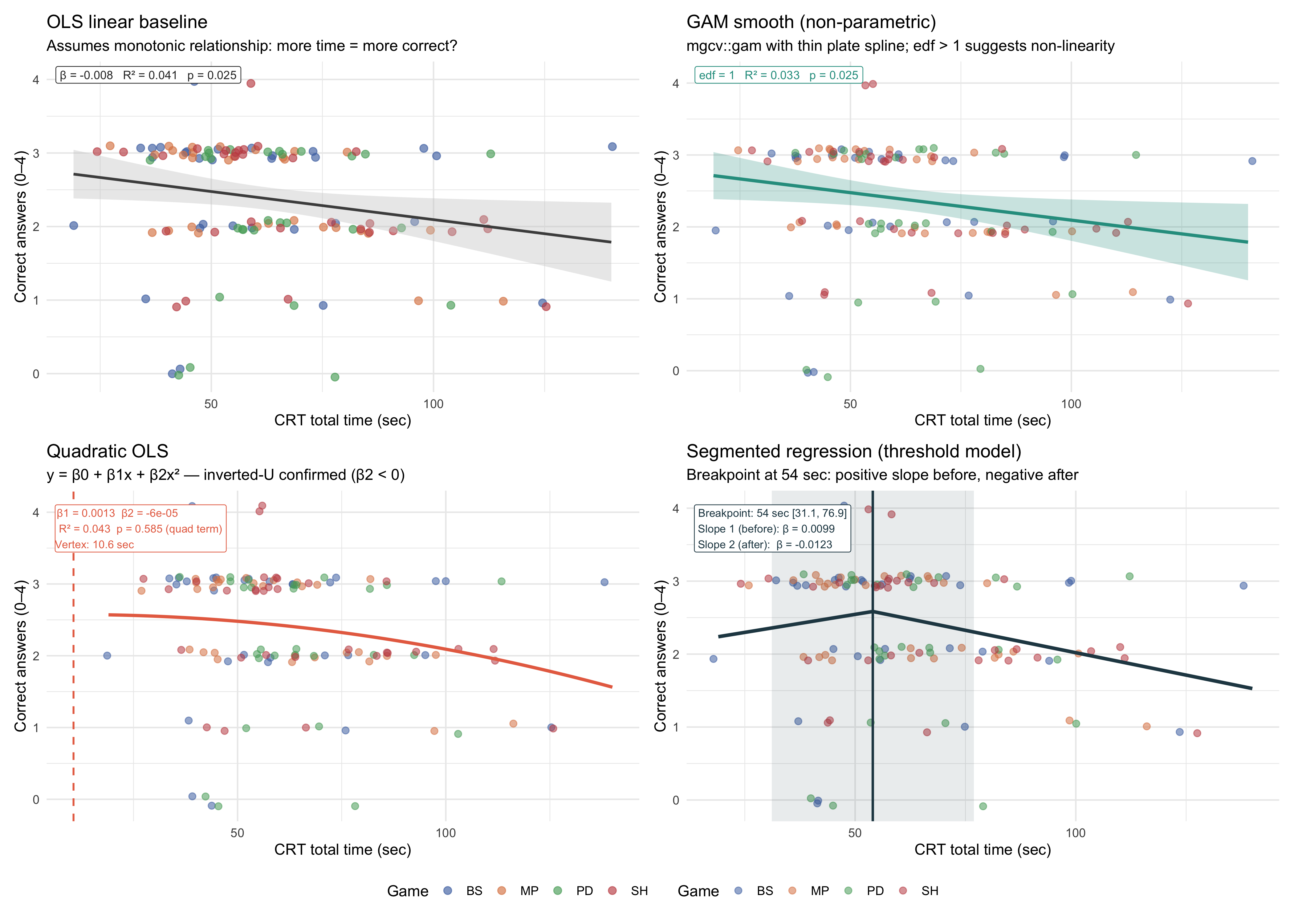
### Summary panel (all four models)
```{r}
#| label: fig-crt-panel
#| fig-cap: "Comparison of four approaches to modelling CRT time → accuracy. Top-left: OLS linear. Top-right: GAM smooth. Bottom-left: Quadratic OLS. Bottom-right: Segmented regression with estimated breakpoint."
#| fig-height: 10
#| fig-width: 14
p_crt_panel
```
## Conditioning on gender and role
::: callout-note
The following analyses condition quiz errors and CRT4 performance on **gender** (Male / Female) and **lab role** (P1 LEEN / P2 CoCoLab) separately — pooled across games. One stratifying variable is shown per plot: no cross-tabulation with `game_id`.
Each violin/boxplot pair is annotated with a **Mann-Whitney U test** (two-sided, unpaired). The stacked-bar perfection charts show a **χ² test** (Monte Carlo p-value, 2000 replicates). Regression models include all three predictors simultaneously (game + gender + role).
:::
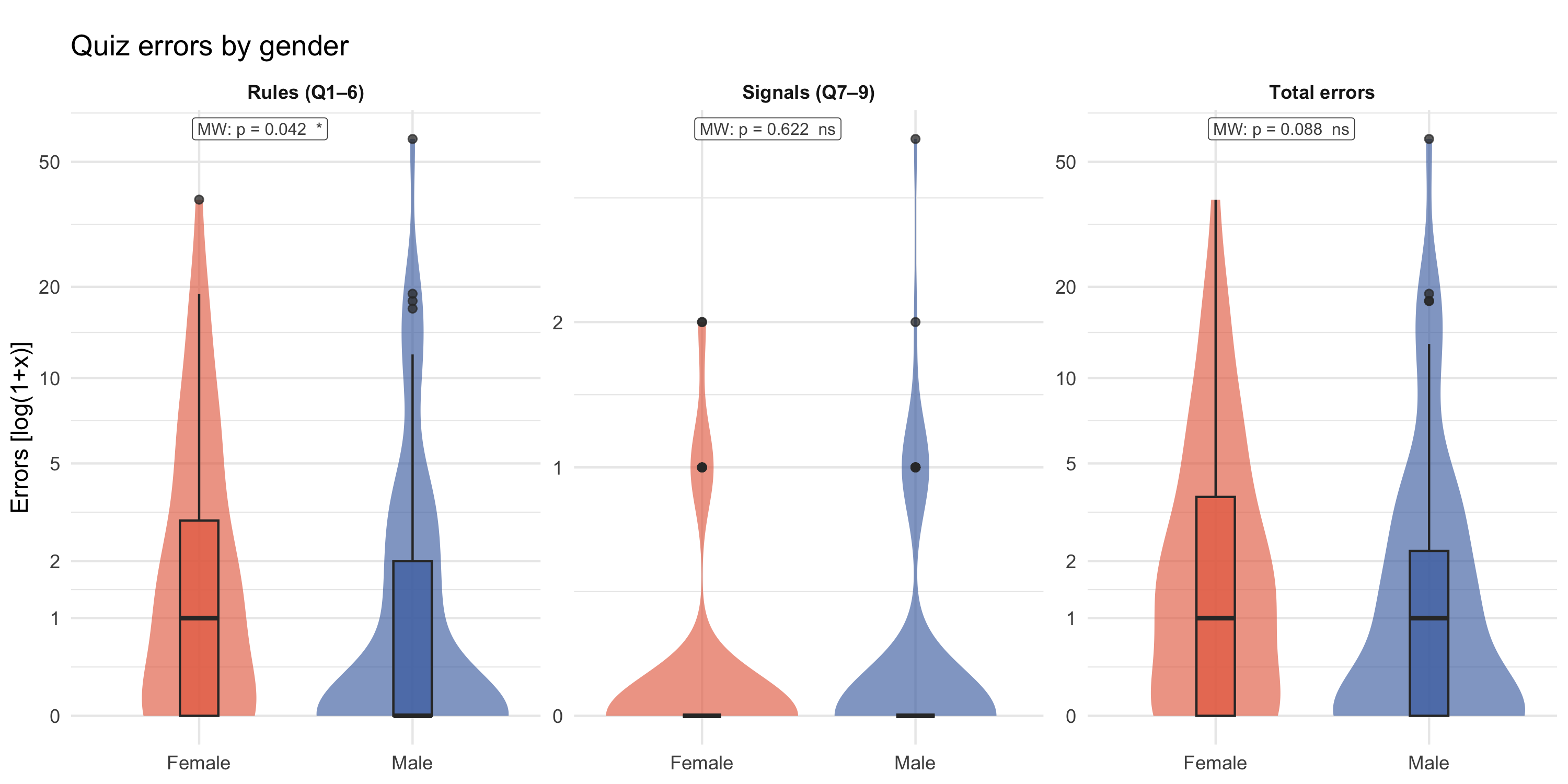
### Quiz errors by gender
```{r}
#| label: fig-quiz-gender
#| fig-cap: "Distribution of quiz errors (rules Q1–6, signals Q7–9, total) by gender [log(1+x) y-axis]. Violin + boxplot overlay, pooled across all games. Tick labels show raw error counts. Mann-Whitney U test p-value shown at the top-left of each panel."
#| fig-height: 5
p_quiz_errors_gender
```
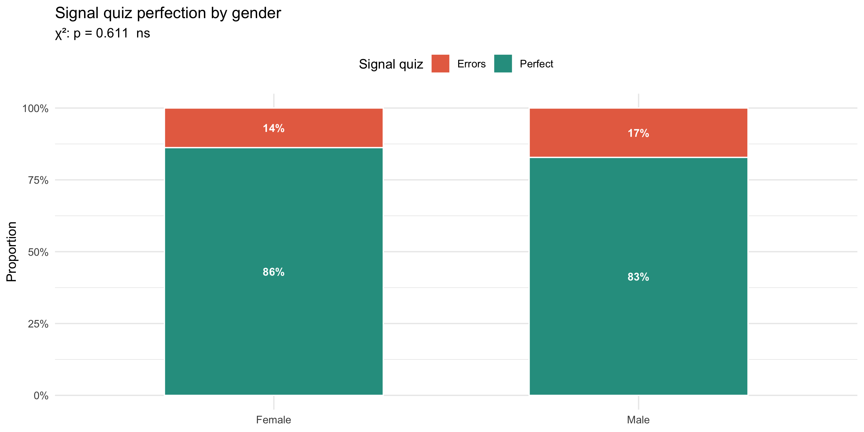
```{r}
#| label: fig-perf-gender
#| fig-cap: "Proportion achieving a perfect signal-quiz score (Q7–9), by gender. χ² test (Monte Carlo) shown in subtitle."
#| fig-height: 5
p_perf_gender
```
### Quiz errors by role
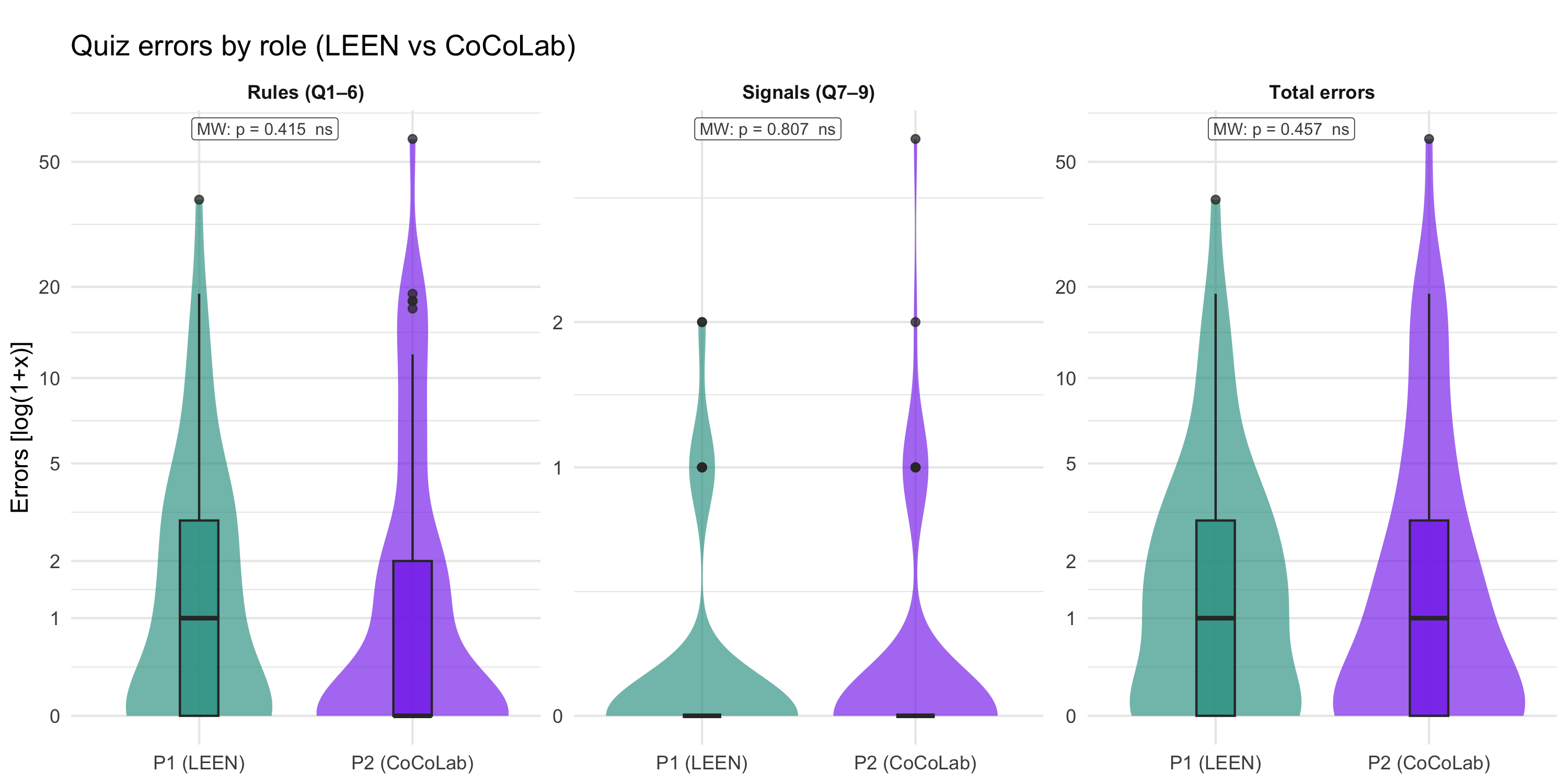
```{r}
#| label: fig-quiz-role
#| fig-cap: "Distribution of quiz errors (rules Q1–6, signals Q7–9, total) by lab role [log(1+x) y-axis]. Violin + boxplot overlay, pooled across all games. Tick labels show raw error counts. Mann-Whitney U test p-value shown at the top-left of each panel."
#| fig-height: 5
p_quiz_errors_role
```
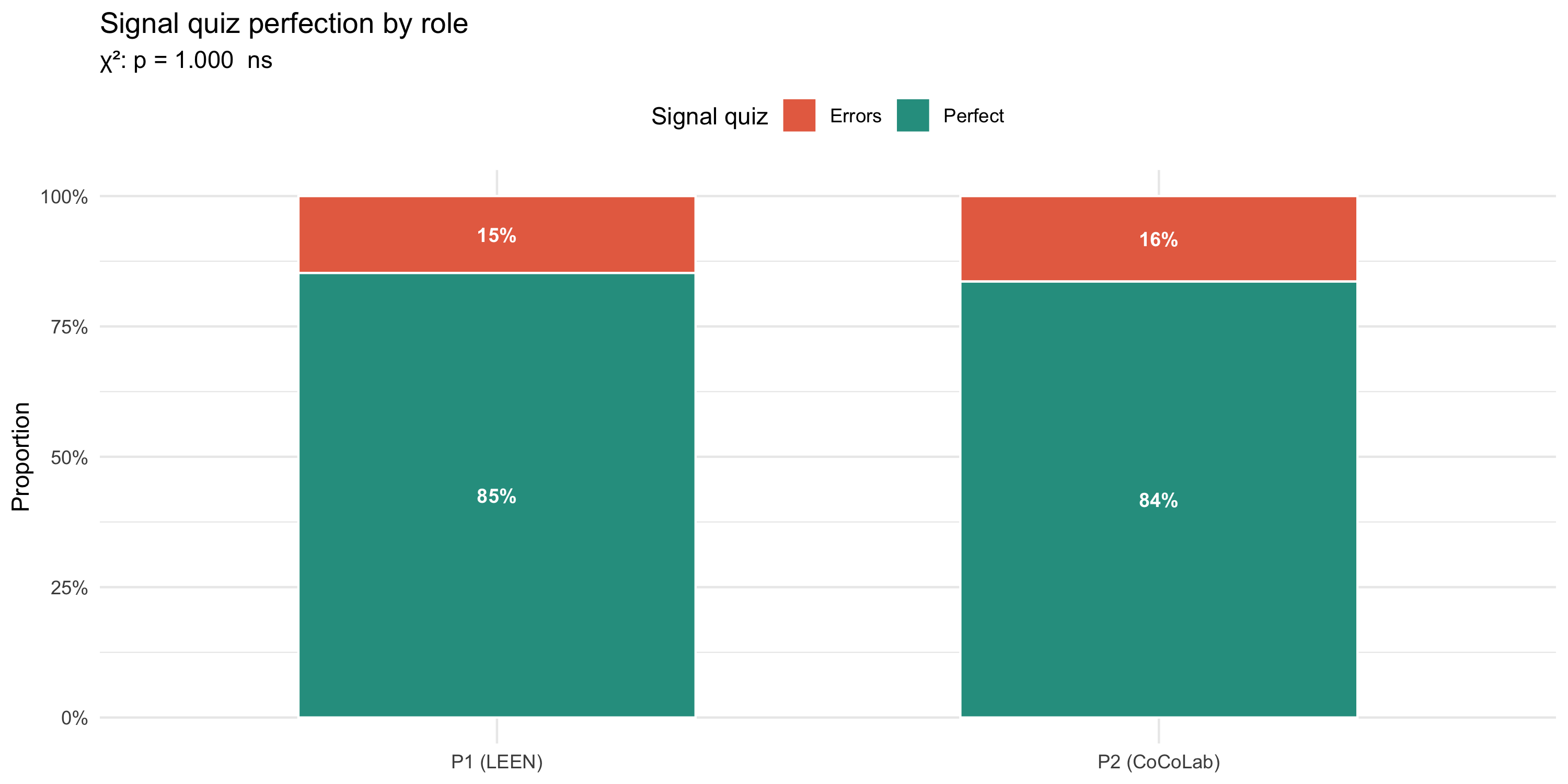
```{r}
#| label: fig-perf-role
#| fig-cap: "Proportion achieving a perfect signal-quiz score, by lab role. χ² test (Monte Carlo) shown in subtitle."
#| fig-height: 5
p_perf_role
```
### CRT4 by gender and role
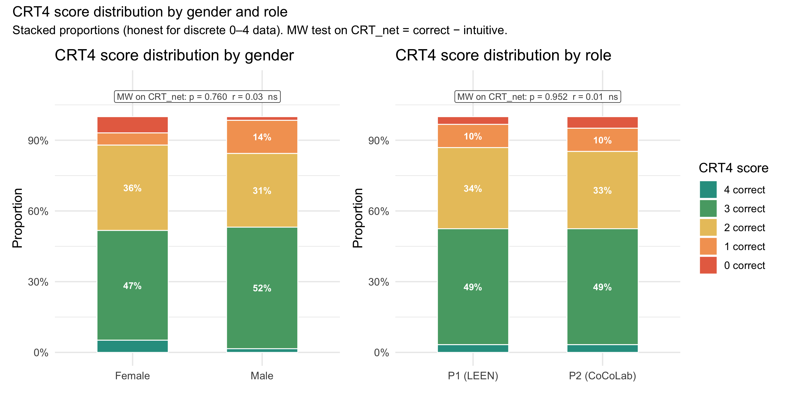
```{r}
#| label: fig-crt4-demo
#| fig-cap: "CRT4 score distribution by gender (left) and by lab role (right). Stacked proportion bars show the share of participants at each discrete score level (0–4): rosso = 0 correct → teal = 4 correct. Labels show % where ≥ 7%. Annotation: Mann-Whitney U on CRT_net = correct − intuitive with rank-biserial r."
#| fig-height: 5
#| fig-width: 10
p_crt4_demo_panel
```
### Regressions with demographic controls
#### Quiz errors — OLS
The table reports OLS estimates of the three quiz-error outcomes regressed simultaneously on game, gender, and role. Reference categories: game = BS, gender = Male, role = P1 (LEEN).
```{r}
#| label: tab-ols8-quiz
gt_ols8_quiz
```
#### CRT4 — binary logistic regression
::: callout-note
CRT4 correct answers take only 5 discrete values (0–4), making OLS inappropriate for inference on a near-bounded outcome. Responses are dichotomised into **high reflectors** (correct ≥ 3) vs **low/intuitive** (correct ≤ 2), and a logistic regression is estimated. Odds ratios > 1 indicate a higher probability of being a high reflector relative to the reference category (BS, Male, LEEN). Wald 95% CIs are reported.
:::
```{r}
#| label: tab-logit8-crt
gt_logit8_crt
```
### Forest plots — partial effects
```{r}
#| label: fig-forest8-rules
#| fig-cap: "OLS β ± 95% CI for each predictor on rules-quiz errors (Q1–6; game + gender + role). Reference: BS, Male, LEEN. Dashed line at zero."
#| fig-height: 5
p_forest8_rules
```
```{r}
#| label: fig-forest8-signals
#| fig-cap: "OLS β ± 95% CI for each predictor on signal-comprehension errors (Q7–9; game + gender + role). Reference: BS, Male, LEEN. Dashed line at zero."
#| fig-height: 5
p_forest8_signals
```
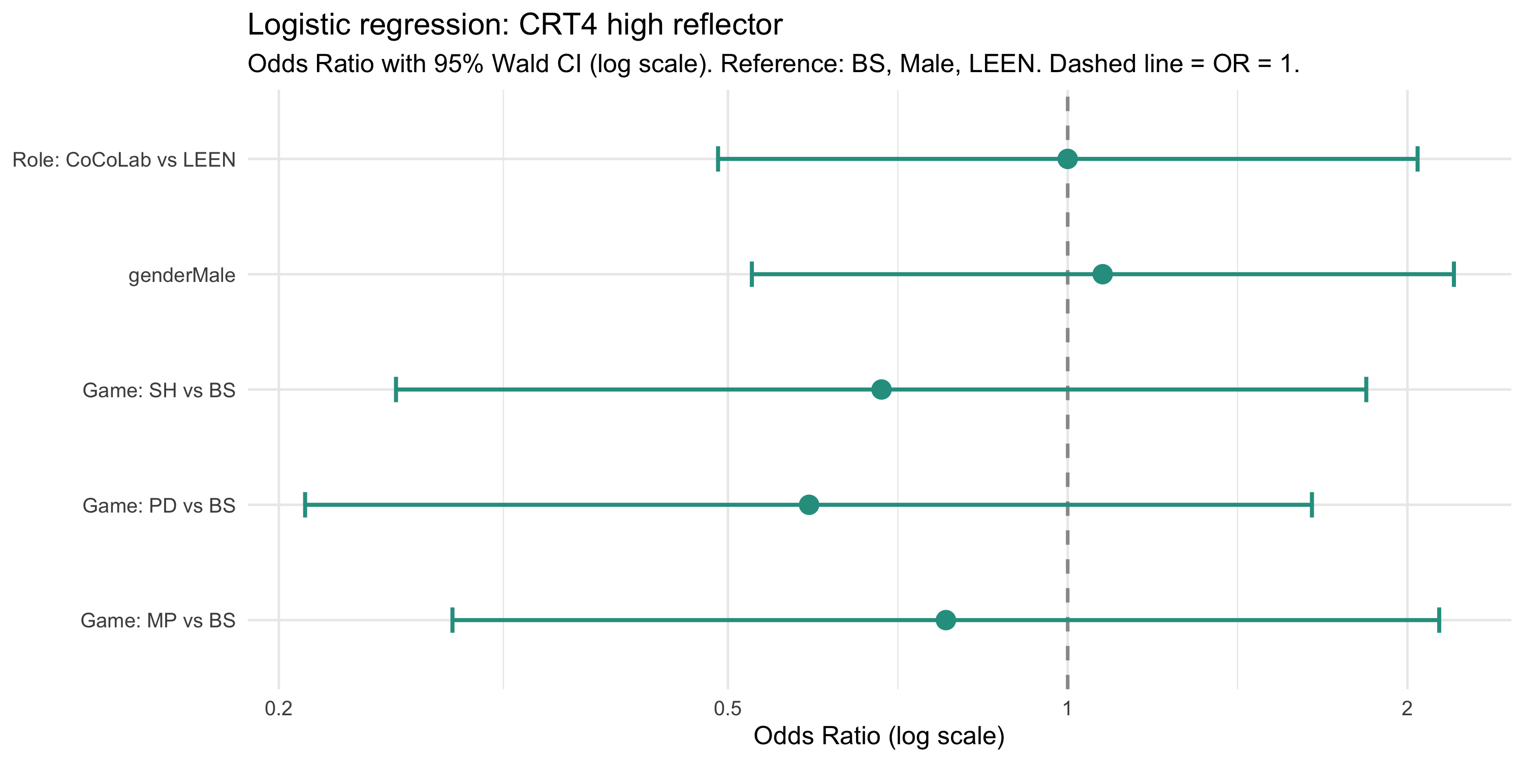
```{r}
#| label: fig-forest8-crt
#| fig-cap: "Logistic regression odds ratios (OR) with 95% Wald CI for CRT4 high-reflector outcome (correct ≥ 3). Log scale: values > 1 = higher odds of being a high reflector; values < 1 = lower odds. Reference: BS, Male, LEEN. Dashed line at OR = 1."
#| fig-height: 5
p_forest8_crt
```
## Preliminary interpretation
```{r}
#| echo: false
pct_perfect <- round(mean(df$quiz_perfect_q7_9, na.rm = TRUE) * 100, 1)
med_errors <- round(median(df$quiz_errors_total, na.rm = TRUE), 0)
med_crt <- round(median(df$CRT_totCorrect_corrected, na.rm = TRUE), 1)
iqr_crt <- round(IQR(df$CRT_totCorrect_corrected, na.rm = TRUE), 1)
cor_rho <- round(cor(df$CRT_totCorrect_corrected, df$quiz_errors_total,
use = "complete.obs", method = "spearman"), 2)
```
**`r pct_perfect`%** of participants answered all signal-comprehension questions correctly. Total errors show the expected right skew (median = `r med_errors`): most participants made few mistakes, but a high-error tail warrants monitoring in robustness checks.
On the CRT4, the sample median is **`r med_crt`** correct answers (IQR = `r iqr_crt`) out of 4. The Spearman correlation between CRT4 score and quiz errors is **ρ = `r cor_rho`** — `r if(cor_rho < -0.1) "a negative association suggesting that more reflective participants also showed better rule comprehension" else if(cor_rho > 0.1) "a positive association — unexpected; examine potential confounds" else "close to zero, indicating the two constructs are largely independent in this sample"`.