---
title: "MASC \u00d7 IRI"
subtitle: "Theory of Mind \u00d7 Empathy \u2014 Cross-instrument analysis · GTEMO Experiment"
author: "Eric Guerci"
date: today
format:
html:
theme: flatly
toc: true
toc-depth: 3
toc-title: "Contents"
number-sections: true
code-fold: true
code-summary: "Show code"
code-tools: true
fig-width: 10
fig-height: 6
fig-dpi: 150
smooth-scroll: true
execute:
echo: true
warning: false
message: false
---
```{r setup}
#| include: false
library(tidyverse)
library(gtsummary)
library(gt)
library(ggplot2)
library(patchwork)
library(scales)
library(rstatix)
library(skimr)
library(psych)
df <- read.csv("../../../data/df_individual_all.csv") |>
mutate(
game_id = factor(game_id, levels = c("BS","MP","PD","SH")),
gender = factor(gender_dummy, levels = c(0, 1), labels = c("Male", "Female")),
role = factor(SINFO_role, levels = c(1, 2), labels = c("P1 (LEEN)", "P2 (CoCoLab)"))
)
col_game <- c("BS" = "#4C72B0", "MP" = "#DD8452",
"PD" = "#55A868", "SH" = "#C44E52")
source("code.R")
```
## Objective
This page tests whether self-reported empathy (**IRI**) is associated with film-based Theory of Mind performance (**MASC**). The two instruments capture related but distinct constructs:
- **MASC** — *implicit, behavioural* ToM measured via naturalistic film clips (17 affective items + 28 cognitive items = 45 total)
- **IRI** — *explicit, self-reported* empathic disposition across four subscales (Perspective Taking, Empathic Concern, Fantasy, Personal Distress)
Two complementary analyses are reported:
1. **Level A — Spearman correlations**: targeted pairings to check whether *matching* pairs (affective ToM ↔ affective empathy; cognitive ToM ↔ cognitive empathy) are stronger than *crossing* ones (discriminant validity)
2. **Level B — Binomial GLMs**: IRI subscales entered simultaneously as predictors of MASC accuracy; a quasi-binomial robustness check corrects for potential overdispersion
```{r}
#| include: false
n_mi <- nrow(df_mi)
```
## Level A — Spearman correlations
```{r}
#| label: tab-spearman
tab_spearman |>
  gt() |>
  cols_label(
    MASC_dim = "MASC dimension",
    Pair     = "Pair",
    rho      = "\u03c1",
    p_fmt    = "p",
    sig      = "Sig."
  ) |>
  tab_header(
    title    = "Spearman correlations: MASC \u00d7 IRI",
    subtitle = paste0("N = ", n_mi,
                      " complete cases. Exact = FALSE (ties present).")
  ) |>
  tab_style(style = cell_text(weight = "bold"),
            locations = cells_column_labels()) |>
  tab_style(style = cell_text(weight = "bold"),
            locations = cells_body(columns = sig, rows = sig != "ns")) |>
  tab_footnote("* p < .05  ** p < .01  *** p < .001  ns = not significant")
```
::: callout-note
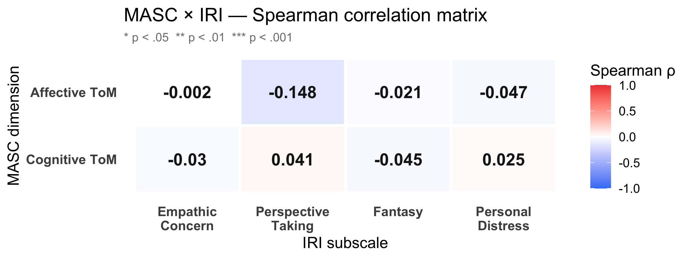
**Matching vs crossing hypothesis.** Affective ToM (emotion inference from film clips) is theorised to align more strongly with affective empathy (Empathic Concern, Personal Distress). Cognitive ToM (belief/intention inference) should align more with cognitive empathy (Perspective Taking). Pairs that cross the affective/cognitive boundary serve as a discriminant validity check — weaker or non-significant ρ there supports construct differentiation.
:::
### Correlation heatmap
```{r}
#| label: fig-cor-heat
#| fig-cap: "Spearman ρ between the two MASC dimensions (rows) and the four IRI subscales (columns). Red = positive association, blue = negative. Significance stars: * p < .05 ** p < .01 *** p < .001."
#| fig-width: 8
#| fig-height: 3
p_cor_heat
```
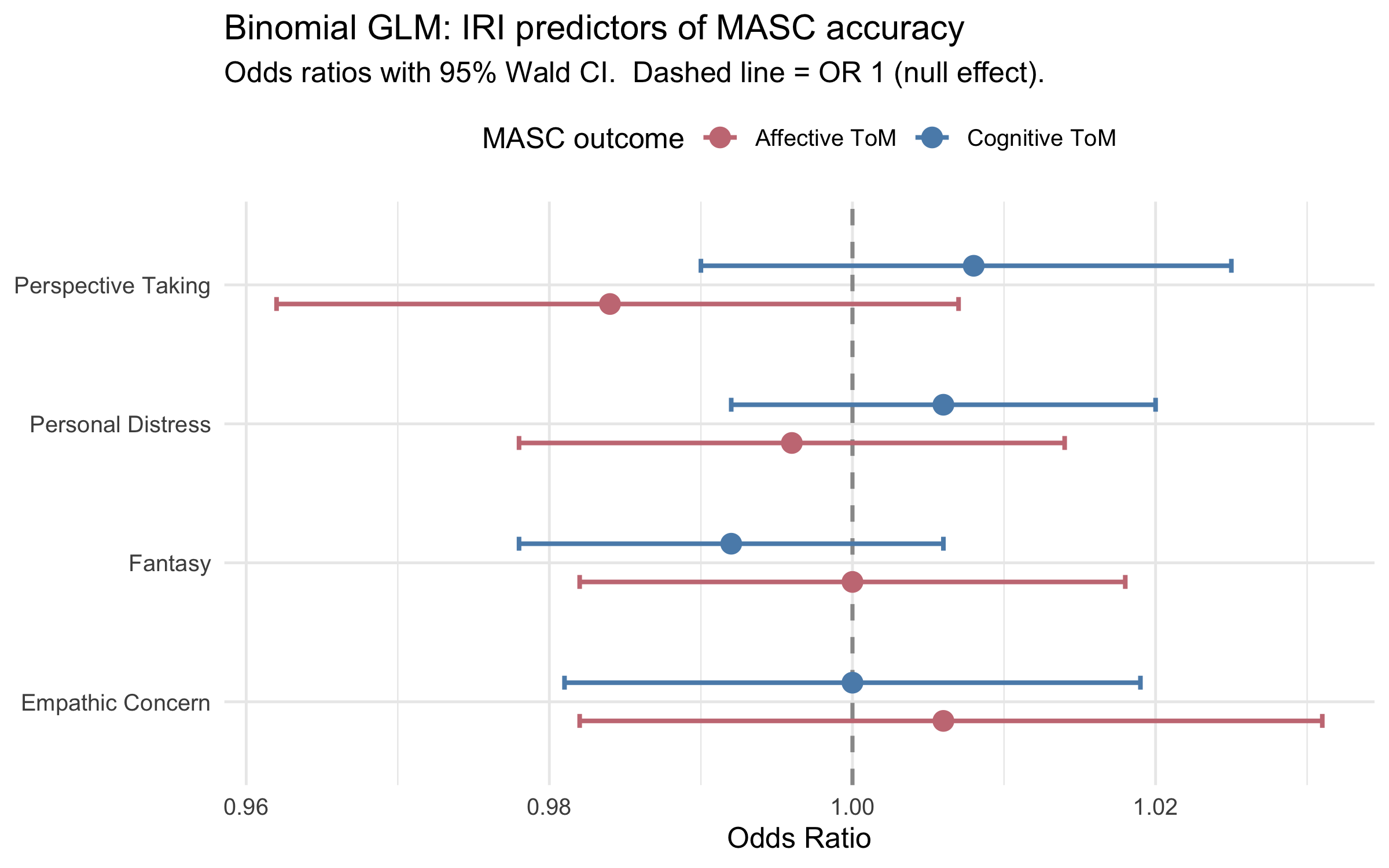
## Level B — Binomial GLMs
IRI subscales entered simultaneously as predictors of MASC accuracy. The response is modelled as a binomial count of correct answers (17 affective items; 28 cognitive items, total = 45). Coefficients are on the log-odds scale; the forest plot shows exponentiated odds ratios (OR) with 95% Wald CIs.
```{r}
#| label: tab-glm
tab_glm |>
  select(Outcome, Predictor, beta, SE, OR, OR_lo, OR_hi, stat, p_fmt, sig) |>
  gt() |>
  tab_header(
    title    = "Binomial GLM: IRI subscales predicting MASC accuracy",
    subtitle = "Family: binomial (logit link). Wald 95% CI."
  ) |>
  cols_label(beta = "\u03b2", SE = "SE", OR = "OR",
             OR_lo = "95% CI lo", OR_hi = "95% CI hi",
             stat = "z", p_fmt = "p", sig = "Sig.") |>
  tab_row_group(label = "Outcome: Cognitive ToM (28 items)",
                rows = Outcome == "Cognitive ToM") |>
  tab_row_group(label = "Outcome: Affective ToM (17 items)",
                rows = Outcome == "Affective ToM") |>
  tab_style(style = cell_text(weight = "bold"),
            locations = cells_column_labels()) |>
  tab_style(style = cell_text(weight = "bold"),
            locations = cells_body(columns = sig, rows = sig != "")) |>
  tab_style(style = cell_text(weight = "bold", color = "#2d7a3a"),
            locations = cells_row_groups()) |>
  tab_footnote("\u03b2 = log-odds coefficient. OR = exp(\u03b2). Wald 95% CI. * p < .05  ** p < .01  *** p < .001.")
```
::: callout-note
**Overdispersion check.** A binomial GLM assumes variance = μ(1−μ)/n; real data often show extra-binomial variation. The dispersion parameter φ is estimated by the quasi-binomial fit: **φ(affective) = `r disp_aff`**, **φ(cognitive) = `r disp_cog`**. φ ≈ 1 means the binomial assumption holds; φ >> 1 means standard binomial SEs are underestimated.
:::
```{r}
#| label: fig-glm-forest
#| fig-cap: "Forest plot: odds ratios from the binomial GLMs. Error bars = 95% Wald CI. Dashed line = OR 1 (null effect)."
#| fig-width: 8
#| fig-height: 5
p_glm_forest
```
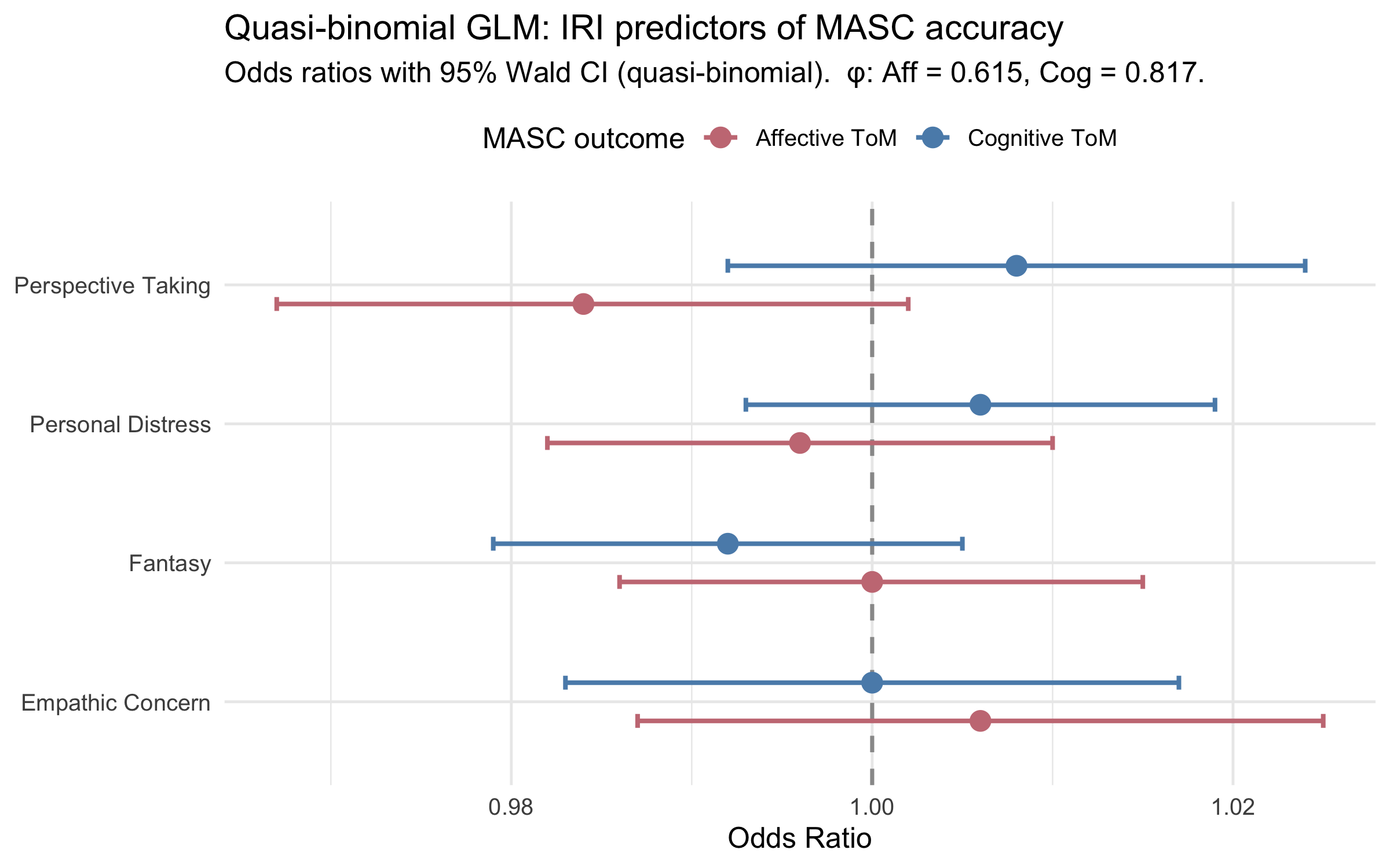
## Quasi-binomial robustness check
The quasi-binomial model uses the same formula but estimates a free dispersion parameter φ, inflating standard errors by √φ. Coefficients (β) and odds ratios are **identical** to the binomial — only SEs and p-values change. The comparison table shows directly where overdispersion changes inference.
```{r}
#| label: tab-glm-compare
tab_glm_compare |>
  select(Outcome, Predictor, beta, OR,
         SE_binom, SE_quasi, SE_ratio,
         p_binom, sig_binom, p_quasi, sig_quasi) |>
  gt() |>
  tab_header(
    title    = "Binomial vs quasi-binomial: SE and p-value comparison",
    subtitle = paste0("\u03c6 (dispersion): Affective = ", disp_aff,
                      ", Cognitive = ", disp_cog,
                      ". SE ratio \u2248 \u221a\u03c6.")
  ) |>
  cols_label(
    beta      = "\u03b2", OR = "OR",
    SE_binom  = "SE (binom)", SE_quasi = "SE (quasi)", SE_ratio = "SE ratio",
    p_binom   = "p (binom)",  sig_binom = "Sig. (binom)",
    p_quasi   = "p (quasi)",  sig_quasi = "Sig. (quasi)"
  ) |>
  tab_row_group(label = "Outcome: Cognitive ToM",
                rows = Outcome == "Cognitive ToM") |>
  tab_row_group(label = "Outcome: Affective ToM",
                rows = Outcome == "Affective ToM") |>
  tab_style(style = cell_text(weight = "bold"),
            locations = cells_column_labels()) |>
  tab_style(style = cell_text(weight = "bold", color = "#2d7a3a"),
            locations = cells_row_groups()) |>
  tab_style(
    style = cell_fill(color = "#fff3cd"),
    locations = cells_body(
      columns = c(sig_binom, sig_quasi),
      rows = sig_binom != sig_quasi
    )
  ) |>
  tab_footnote("Yellow highlight = significance changes between models. SE ratio = SE\u2098\u1d64\u1d43\u02e2\u1d35 / SE\u1d47\u1d35\u207f\u1d52\u1d50.")
```
```{r}
#| label: fig-glm-forest-quasi
#| fig-cap: "Forest plot: odds ratios from the quasi-binomial GLMs. Wider CIs reflect SE inflation by √φ. Compare with the binomial forest plot above."
#| fig-width: 8
#| fig-height: 5
p_glm_forest_quasi
```