---
title: "MASC (ToM)"
subtitle: "Movie for the Assessment of Social Cognition · GTEMO Experiment"
author: "Eric Guerci"
date: today
format:
html:
theme: flatly
toc: true
toc-depth: 3
toc-title: "Contents"
number-sections: true
code-fold: true
code-summary: "Show code"
code-tools: true
fig-width: 10
fig-height: 6
fig-dpi: 150
smooth-scroll: true
execute:
echo: true
warning: false
message: false
---
```{r setup}
#| include: false
library(tidyverse)
library(gtsummary)
library(gt)
library(ggplot2)
library(patchwork)
library(scales)
library(rstatix)
library(skimr)
library(psych)
df <- read.csv("../../../data/df_individual_all.csv") |>
mutate(
game_id = factor(game_id, levels = c("BS","MP","PD","SH")),
gender = factor(gender_dummy, levels = c(0, 1), labels = c("Male", "Female")),
role = factor(SINFO_role, levels = c(1, 2), labels = c("P1 (LEEN)", "P2 (CoCoLab)"))
)
col_game <- c("BS" = "#4C72B0", "MP" = "#DD8452",
"PD" = "#55A868", "SH" = "#C44E52")
source("code.R")
```
## Background
**Theory of Mind (ToM)** is the ability to attribute mental states — beliefs, intentions, desires, emotions — to others and to understand that these may differ from one's own. It is a core dimension of social cognition and underlies strategic behaviour in interactive settings: anticipating what others know, want, and believe is a prerequisite for effective communication, negotiation, and cooperation.
The **Movie for the Assessment of Social Cognition (MASC)** is a validated film-based instrument developed by Dziobek et al. (2006). Participants watch short video clips of social interactions and answer multiple-choice questions about the characters' thoughts and feelings. The MASC is designed to capture *ecological* ToM by embedding mental-state inference in naturalistic, dynamic social scenes — closer to real-world interaction than classic vignette-based tasks.
The instrument yields five scores:
| Variable | Description | Scale |
|----------|-------------|-------|
| `MASC_ToM_score` | Total correct ToM responses | 0 – 45 |
| `MASC_dimToM_score` | *Diminishing* errors — under-mentalising | 0 – 45 |
| `MASC_excToM_score` | *Exceeding* errors — over-mentalising | 0 – 45 |
| `MASC_noToM_score` | *No ToM* errors — no mental-state attribution | 0 – 45 |
| `MASC_attention_score` | Correct attention-check items (control) | 0 – 6 |
Items are further classified as **affective** (emotion inference, 17 items) or **cognitive** (belief/intention inference, 28 items), yielding two proportion scores (`MASC_affective_perc_score`, `MASC_cognitive_perc_score`) that allow dissociation of the two ToM components.
## Data overview
```{r}
#| label: masc-overview
#| tbl-cap: "Descriptive skim of MASC variables including the attention control score."
df |>
  select(game_id,
         MASC_ToM_score, MASC_dimToM_score, MASC_excToM_score,
         MASC_noToM_score, MASC_attention_score,
         MASC_affective_perc_score, MASC_cognitive_perc_score) |>
  skim()
```
## Descriptive statistics by game
```{r}
#| label: tab-masc
tab_masc
```
::: callout-note
Statistics are median (Q1, Q3). The Kruskal-Wallis test checks whether distributions differ across the 4 games; η² quantifies the effect size (small ≥ 0.01, medium ≥ 0.06, large ≥ 0.14). A significant p indicates heterogeneity in ToM profiles across games — relevant for interpreting group-level strategic differences in the behaviour sections.
:::
## Affective vs cognitive ToM
### Sample-level summary
```{r}
#| label: aff-cog-summary
df |>
  select(`Affective ToM` = MASC_affective_perc_score,
         `Cognitive ToM` = MASC_cognitive_perc_score) |>
  pivot_longer(everything(), names_to = "Dimension", values_to = "score") |>
  group_by(Dimension) |>
  summarise(
    Median = median(score, na.rm = TRUE),
    Q1     = quantile(score, 0.25, na.rm = TRUE),
    Q3     = quantile(score, 0.75, na.rm = TRUE),
    .groups = "drop"
  ) |>
  gt() |>
  fmt_number(columns = c(Median, Q1, Q3), decimals = 3) |>
  tab_header(title = "Affective vs Cognitive ToM: sample-level summary (median, IQR)")
```
The following tests whether affective and cognitive ToM accuracy differ within individuals (paired Wilcoxon signed-rank, as scores are bounded proportions).
```{r}
#| label: aff-cog-test
tibble(
  Statistic      = c("V (Wilcoxon)", "p-value", "Pseudo-median diff. (H-L)",
                     "95% CI lower", "95% CI upper",
                     "Effect size r", "Magnitude"),
  Value          = c(
    round(wilcox_res$statistic,  1),
    signif(wilcox_res$p.value,   3),
    round(wilcox_res$estimate,   4),
    round(wilcox_res$conf.int[1],4),
    round(wilcox_res$conf.int[2],4),
    round(wilcox_es$effsize,     3),
    as.character(wilcox_es$magnitude)
  )
) |>
  gt() |>
  tab_header(
    title    = "Wilcoxon signed-rank: Affective vs Cognitive ToM",
    subtitle = "Pseudo-median difference = Hodges-Lehmann estimator (Affective \u2212 Cognitive)"
  ) |>
  tab_style(style = cell_text(weight = "bold"),
            locations = cells_column_labels())
```
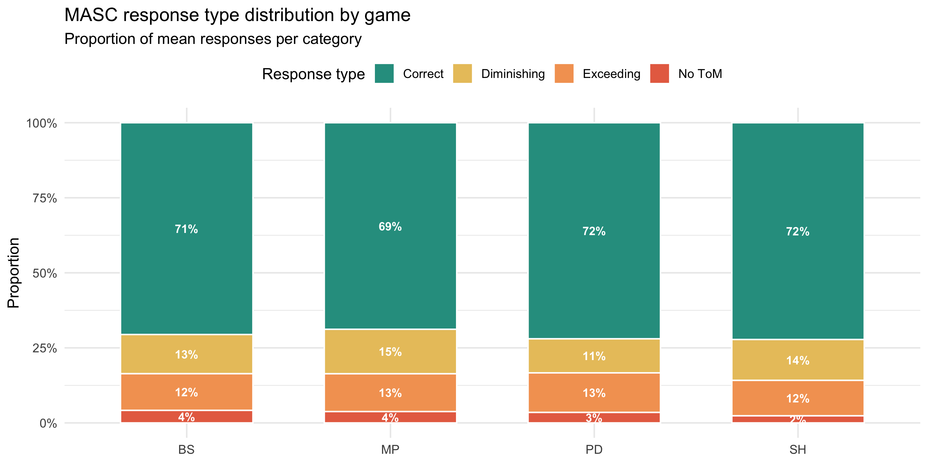
## Figures
### Response type distribution
```{r}
#| label: fig-stacked
#| fig-cap: "Average proportion of the 4 MASC response types per experimental condition. Correct responses dominate; diminishing (under-mentalising) is the most frequent error type, consistent with non-clinical samples."
#| fig-height: 5
p_stacked
```
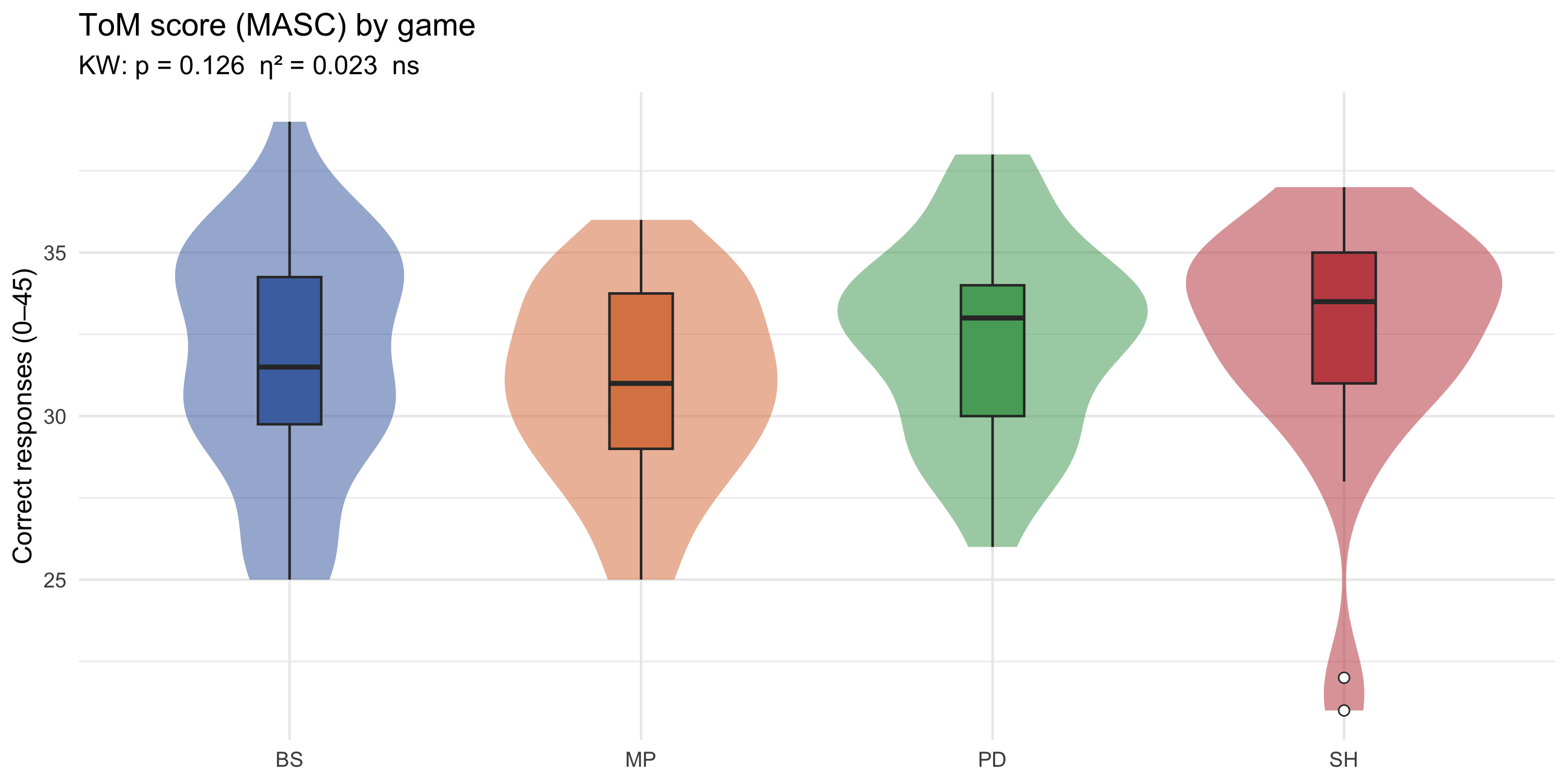
### ToM score distribution by game
```{r}
#| label: fig-violin-tom
#| fig-cap: "Distribution of total correct ToM score (0–45) by experimental condition."
#| fig-height: 5
p_violin_tom
```
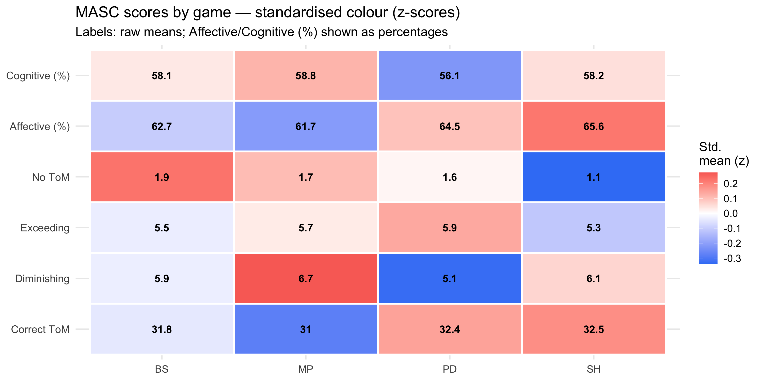
### MASC dimensions heatmap
```{r}
#| label: fig-heatmap
#| fig-cap: "Within-variable standardised means (z-scores) across games — colour encodes relative position within each dimension. Cell labels show raw means; Affective (%) and Cognitive (%) labels are multiplied ×100 for readability."
#| fig-height: 5
p_heat_masc
```
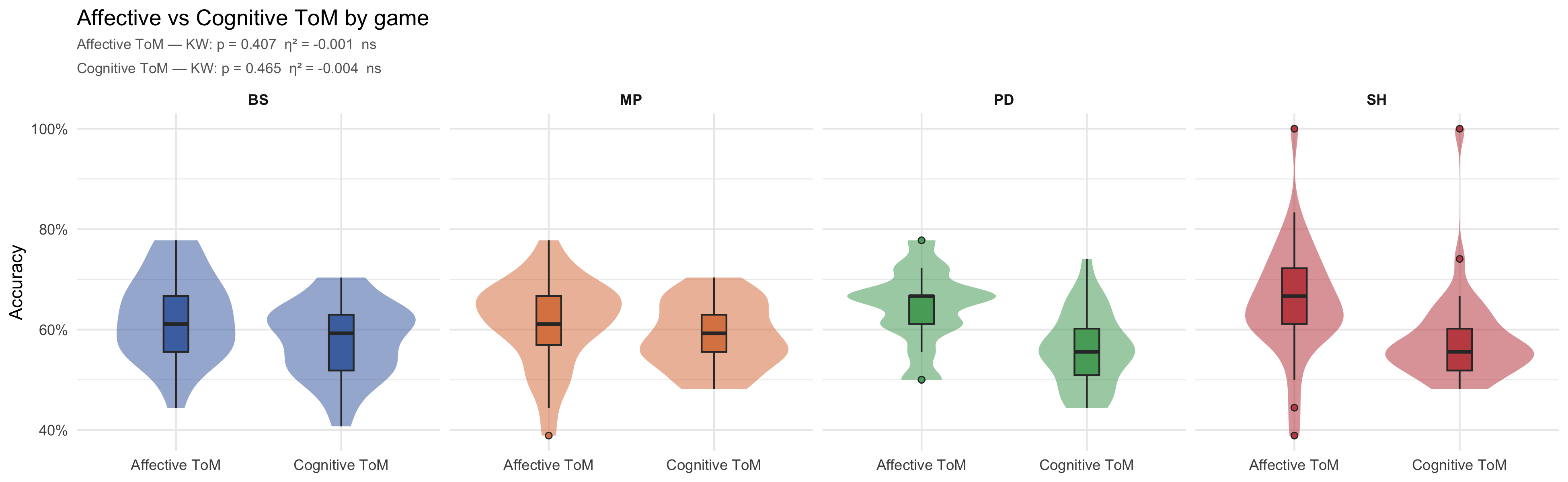
### Affective vs Cognitive ToM by game
```{r}
#| label: fig-aff-cog
#| fig-cap: "Distributions of affective and cognitive ToM accuracy by experimental condition. Accuracy displayed as proportion (0–1). Subtitles report Kruskal-Wallis tests (η²) across the 4 game conditions separately for each ToM dimension."
#| fig-width: 13
#| fig-height: 4
p_aff_cog
```
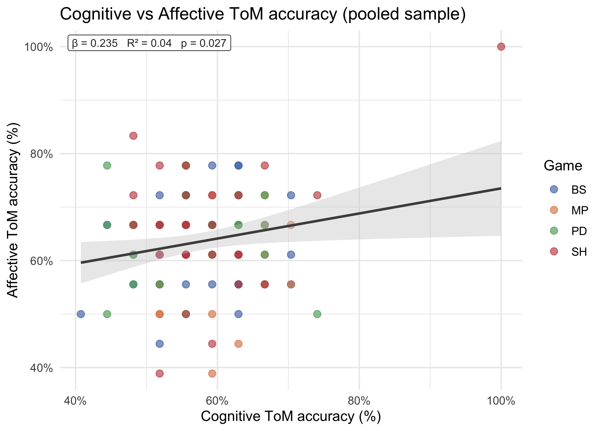
### Cognitive vs affective ToM scatter (pooled sample)
```{r}
#| label: fig-scatter
#| fig-cap: "Pooled scatter of cognitive vs affective ToM accuracy with a single OLS regression line (grey). The top-left label reports β, R², and significance. Points coloured by game."
#| fig-width: 7
#| fig-height: 5
p_scatter
```
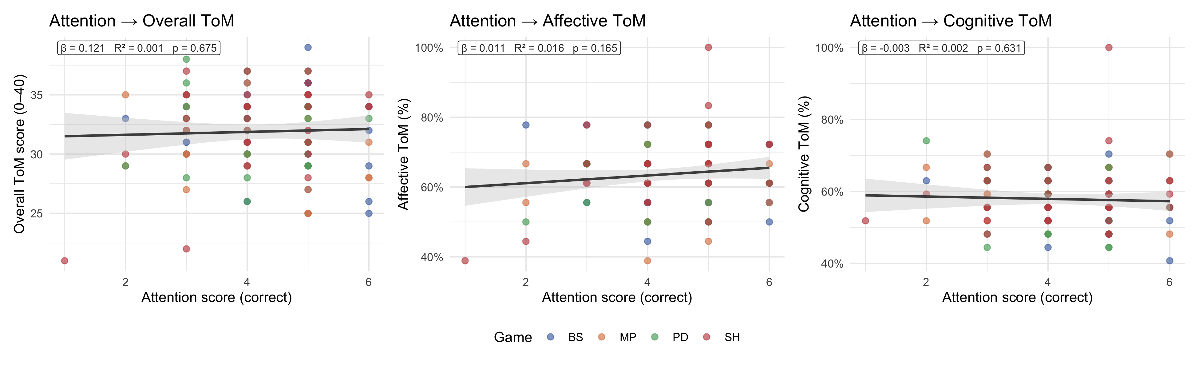
### Attention control vs ToM scores
The MASC includes attention-check items that do not require mental-state inference. Correlating the attention score with ToM scores helps assess whether performance differences are driven by general task engagement rather than ToM ability per se.
```{r}
#| label: fig-attention
#| fig-cap: "Scatter plots of the MASC attention-check score against overall ToM score (left), affective ToM accuracy (centre), and cognitive ToM accuracy (right). OLS line with 95% CI; annotation reports β, R², p-value. Points coloured by game."
#| fig-width: 13
#| fig-height: 4
p_attention_panel
```
::: callout-note
A strong positive association between attention score and ToM scores would indicate that overall task engagement (rather than ToM specifically) drives performance. A weak or absent association is more consistent with ToM scores reflecting the construct of interest.
:::
## Conditioning on gender and role
::: callout-note
Distributions stratified by gender and role, followed by OLS models with game, gender, and role entered simultaneously. Reference category: game = BS, gender = Male, role = P1 (LEEN).
:::
### MASC by gender and role (pooled)
```{r}
#| label: fig-masc-cond-pooled
#| fig-cap: "MASC overall ToM score by gender (left) and experimental role (right), pooled across game conditions. Mann-Whitney U test with rank-biserial r effect size."
#| fig-width: 10
#| fig-height: 5
p_masc_cond_pooled
```
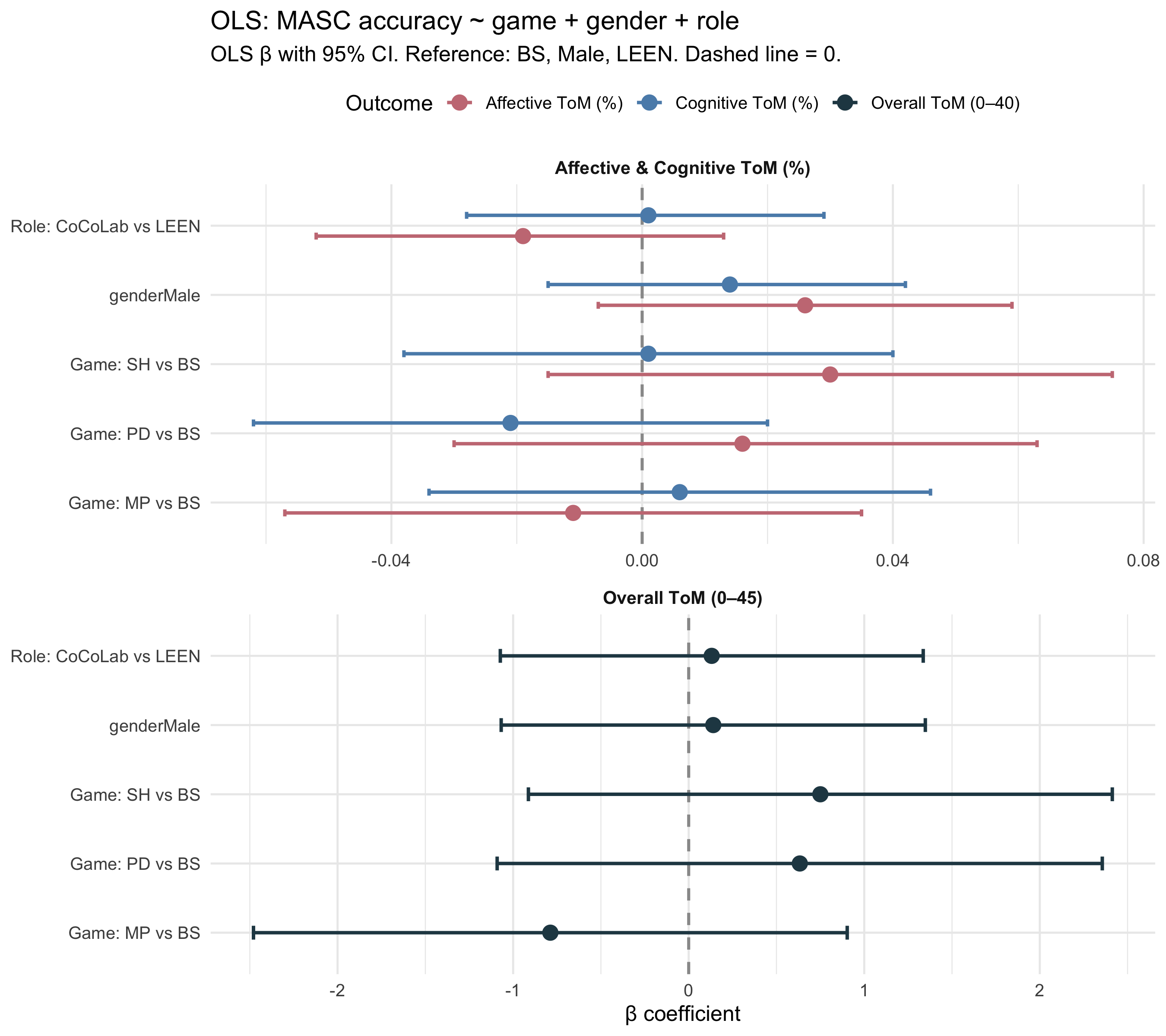
### OLS with demographic controls
```{r}
#| label: tab-ols-masc
gt_ols_masc
```
```{r}
#| label: fig-forest-masc8
#| fig-cap: "Forest plot: OLS β with 95% CI for MASC outcomes (game + gender + role). Top panel: Overall ToM (0–45 scale); bottom panel: Affective ToM and Cognitive ToM overlaid (both proportion scale, 0–1). Free x-axis per panel. Dashed line = 0."
#| fig-width: 9
#| fig-height: 8
p_forest_masc8
```
::: callout-note
**Interpretation.** Game coefficients represent the conditional effect of game assignment given equal gender and role composition. A game effect that is significant unconditionally (Kruskal-Wallis) but non-significant here suggests partial confounding by demographics.
:::
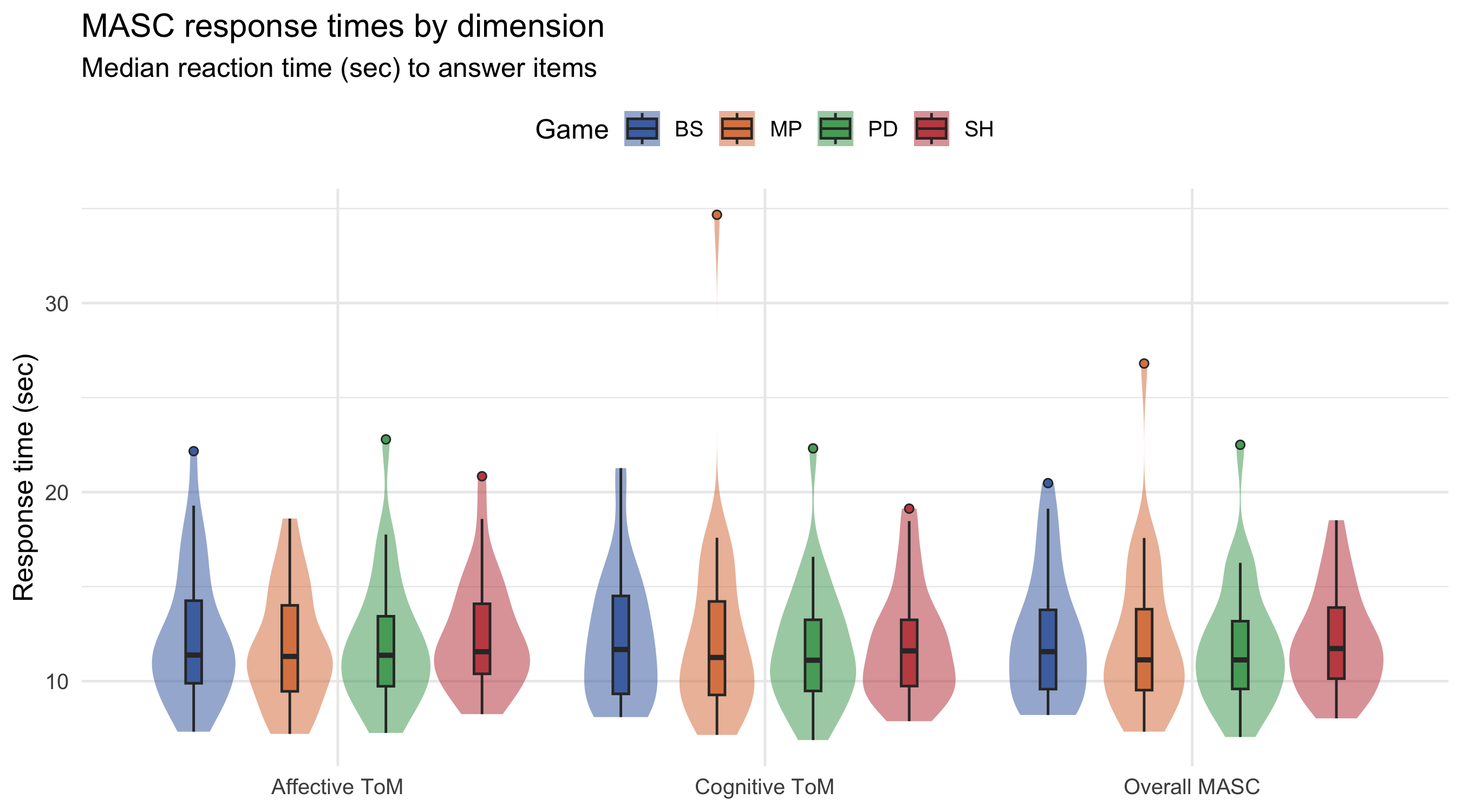
## Response times
### MASC response times by dimension
```{r}
#| label: tab-resp-times
tab_resp_times
```
### Speed–accuracy trade-off
```{r}
#| label: fig-masc-rt-violin
#| fig-cap: "Distribution of MASC response times by dimension (overall / affective / cognitive) across games. Faster response times may reflect overconfidence or heuristic use; slower times suggest deliberative mentalising."
#| fig-width: 9
#| fig-height: 5
p_masc_rt
```
```{r}
#| label: fig-masc-rt-cond
#| fig-cap: "MASC average response times (Overall / Affective / Cognitive) by gender (top) and experimental role (bottom), pooled across game conditions. Mann-Whitney U test with rank-biserial r annotated per facet."
#| fig-width: 11
#| fig-height: 9
p_masc_rt_cond
```
::: callout-note
**Response time differences by gender and role.** A significant Mann-Whitney result would indicate that one group responds systematically faster or slower across MASC dimensions — potentially reflecting differences in deliberative mentalising strategies, not just accuracy. Results should be interpreted alongside the ToM score conditioning (see § Conditioning on gender and role).
:::
## Preliminary interpretation
```{r}
#| echo: false
med_tom <- round(median(df$MASC_ToM_score, na.rm = TRUE), 1)
iqr_tom <- round(IQR(df$MASC_ToM_score, na.rm = TRUE), 1)
med_aff <- round(median(df$MASC_affective_perc_score, na.rm = TRUE), 3)
med_cog <- round(median(df$MASC_cognitive_perc_score, na.rm = TRUE), 3)
wil_p <- signif(wilcox_res$p.value, 2)
wil_es <- round(wilcox_es$effsize, 2)
wil_mag <- as.character(wilcox_es$magnitude)
```
The sample shows a median MASC ToM score of **`r med_tom`** (IQR = `r iqr_tom`) out of 40 items, consistent with adequate mentalising ability in a non-clinical adult population. The affective component (median `r med_aff*100`%) and the cognitive component (median `r med_cog*100`%) are compared within individuals: the Wilcoxon signed-rank test yields p = `r wil_p`, with a `r wil_mag` effect size (r = `r wil_es`), suggesting `r if(wil_p < 0.05) "a statistically significant" else "no significant"` difference between the two ToM dimensions at the sample level.
Differences in MASC profiles across games are informative to the extent that randomisation was imperfect or that participant sorting occurred. Any significant Kruskal-Wallis effects will be noted as potential covariates in the inferential sections.