---
title: "Ib — Theory of Mind (MASC) & Empathy (IRI): descriptive analysis"
subtitle: "Descriptive Analyses · GTEMO Experiment"
author: "Eric Guerci"
date: today
format:
html:
theme: flatly
toc: true
toc-depth: 3
toc-title: "Contents"
number-sections: true
code-fold: true
code-summary: "Show code"
code-tools: true
fig-width: 10
fig-height: 6
fig-dpi: 150
smooth-scroll: true
execute:
echo: true
warning: false
message: false
---
```{r setup}
#| include: false
library(tidyverse)
library(gtsummary)
library(gt)
library(ggplot2)
library(patchwork)
library(scales)
library(rstatix)
library(skimr)
library(psych)
df <- read.csv("../../../data/df_individual_all.csv") |>
mutate(game_id = factor(game_id, levels = c("BS","MP","PD","SH")))
col_game <- c("BS" = "#4C72B0", "MP" = "#DD8452",
"PD" = "#55A868", "SH" = "#C44E52")
source("code.R")
```
## Background
### Theory of Mind and the MASC
**Theory of Mind (ToM)** is the ability to attribute mental states — beliefs, intentions, desires, emotions — to others and to understand that these may differ from one's own. It is a core dimension of social cognition and underlies strategic behaviour in interactive settings: anticipating what others know, want, and believe is a prerequisite for effective communication, negotiation, and cooperation.
The **Movie for the Assessment of Social Cognition (MASC)** is a validated film-based instrument developed by Dziobek et al. (2006). Participants watch short video clips of social interactions and answer multiple-choice questions about the characters' thoughts and feelings. The MASC is designed to capture *ecological* ToM by embedding mental-state inference in naturalistic, dynamic social scenes — closer to real-world interaction than classic vignette-based tasks.
The instrument yields five scores:
| Variable | Description | Scale |
|----------|-------------|-------|
| `MASC_ToM_score` | Total correct ToM responses | 0 – 40 |
| `MASC_dimToM_score` | *Diminishing* errors — under-mentalising | 0 – 36 |
| `MASC_excToM_score` | *Exceeding* errors — over-mentalising | 0 – 36 |
| `MASC_noToM_score` | *No ToM* errors — no mental-state attribution | 0 – 36 |
| `MASC_attention_score` | Correct attention-check items (control) | 0 – 15 |
Items are further classified as **affective** (emotion inference) or **cognitive** (belief/intention inference), yielding two proportion scores (`MASC_affective_perc_score`, `MASC_cognitive_perc_score`) that allow dissociation of the two ToM components.
### Interpersonal Reactivity Index (IRI)
The **IRI** (Davis, 1983) is the standard multi-dimensional self-report measure of empathy. It distinguishes between cognitive and affective aspects of empathy across four subscales (each 0–28):
| Subscale | Description |
|----------|-------------|
| `IRI_perspectiveTaking` | Cognitive: spontaneous tendency to adopt others' point of view |
| `IRI_empathicConcern` | Affective: other-oriented feelings of warmth and concern |
| `IRI_fantasy` | Tendency to imaginatively transpose into fictional characters |
| `IRI_personalDistress` | Self-oriented distress in response to others' suffering |
The IRI is analysed here alongside the MASC because both instruments tap social-cognitive ability (albeit via different channels — implicit film-based behaviour vs explicit self-report), and both may moderate strategic behaviour in the GTEMO games.
## Data overview
```{r}
#| label: masc-overview
#| tbl-cap: "Descriptive skim of MASC variables including the attention control score."
df |>
  select(game_id,
         MASC_ToM_score, MASC_dimToM_score, MASC_excToM_score,
         MASC_noToM_score, MASC_attention_score,
         MASC_affective_perc_score, MASC_cognitive_perc_score) |>
  skim()
```
## MASC analysis
### Descriptive statistics by game
```{r}
#| label: tab-masc
tab_masc
```
::: callout-note
Statistics are median (Q1, Q3). The Kruskal-Wallis test checks whether distributions differ across the 4 games; η² quantifies the effect size (small ≥ 0.01, medium ≥ 0.06, large ≥ 0.14). A significant p indicates heterogeneity in ToM profiles across games — relevant for interpreting group-level strategic differences in Parts II–III.
:::
### Affective vs cognitive ToM comparison
```{r}
#| label: aff-cog-summary
df |>
  select(`Affective ToM` = MASC_affective_perc_score,
         `Cognitive ToM` = MASC_cognitive_perc_score) |>
  pivot_longer(everything(), names_to = "Dimension", values_to = "score") |>
  group_by(Dimension) |>
  summarise(
    Median = median(score, na.rm = TRUE),
    Q1     = quantile(score, 0.25, na.rm = TRUE),
    Q3     = quantile(score, 0.75, na.rm = TRUE),
    .groups = "drop"
  ) |>
  gt() |>
  fmt_number(columns = c(Median, Q1, Q3), decimals = 3) |>
  tab_header(title = "Affective vs Cognitive ToM: sample-level summary (median, IQR)")
```
The following tests whether, at the sample level, affective and cognitive ToM accuracy differ within individuals (paired Wilcoxon signed-rank, as scores are bounded proportions).
```{r}
#| label: aff-cog-test
# Results computed in code.R: wilcox_res (Hodges-Lehmann CI) + wilcox_es (effect size r)
tibble(
  Statistic      = c("V (Wilcoxon)", "p-value", "Pseudo-median diff. (H-L)",
                     "95% CI lower", "95% CI upper",
                     "Effect size r", "Magnitude"),
  Value          = c(
    round(wilcox_res$statistic,  1),
    signif(wilcox_res$p.value,   3),
    round(wilcox_res$estimate,   4),
    round(wilcox_res$conf.int[1],4),
    round(wilcox_res$conf.int[2],4),
    round(wilcox_es$effsize,     3),
    as.character(wilcox_es$magnitude)
  )
) |>
  gt() |>
  tab_header(
    title    = "Wilcoxon signed-rank: Affective vs Cognitive ToM",
    subtitle = "Pseudo-median difference = Hodges-Lehmann estimator (Affective − Cognitive)"
  ) |>
  tab_style(style = cell_text(weight = "bold"),
            locations = cells_column_labels())
```
## Figures — MASC
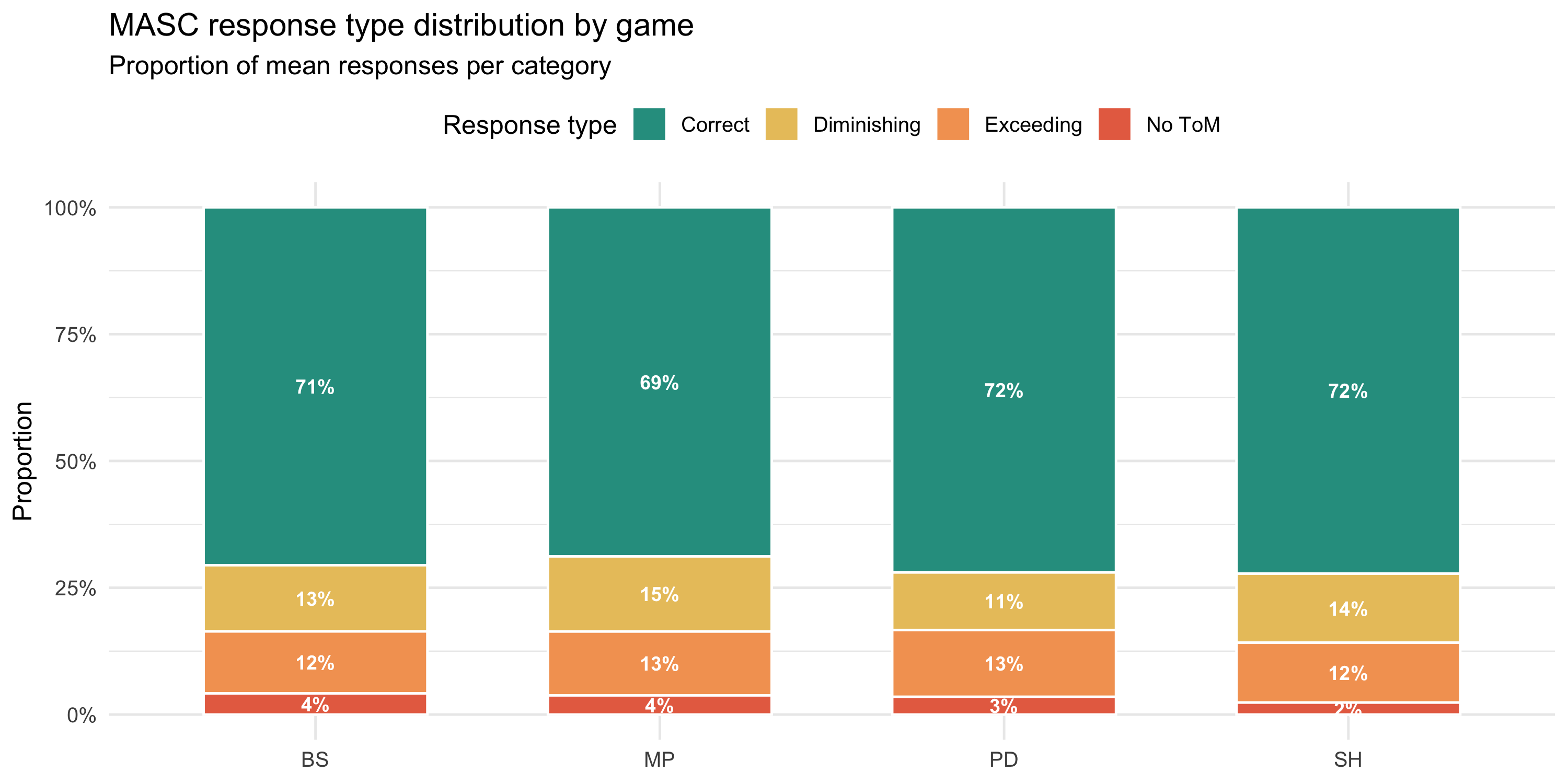
### Response type distribution
```{r}
#| label: fig-stacked
#| fig-cap: "Average proportion of the 4 MASC response types per experimental condition. Correct responses dominate; diminishing (under-mentalising) is the most frequent error type, consistent with non-clinical samples."
#| fig-height: 5
p_stacked
```
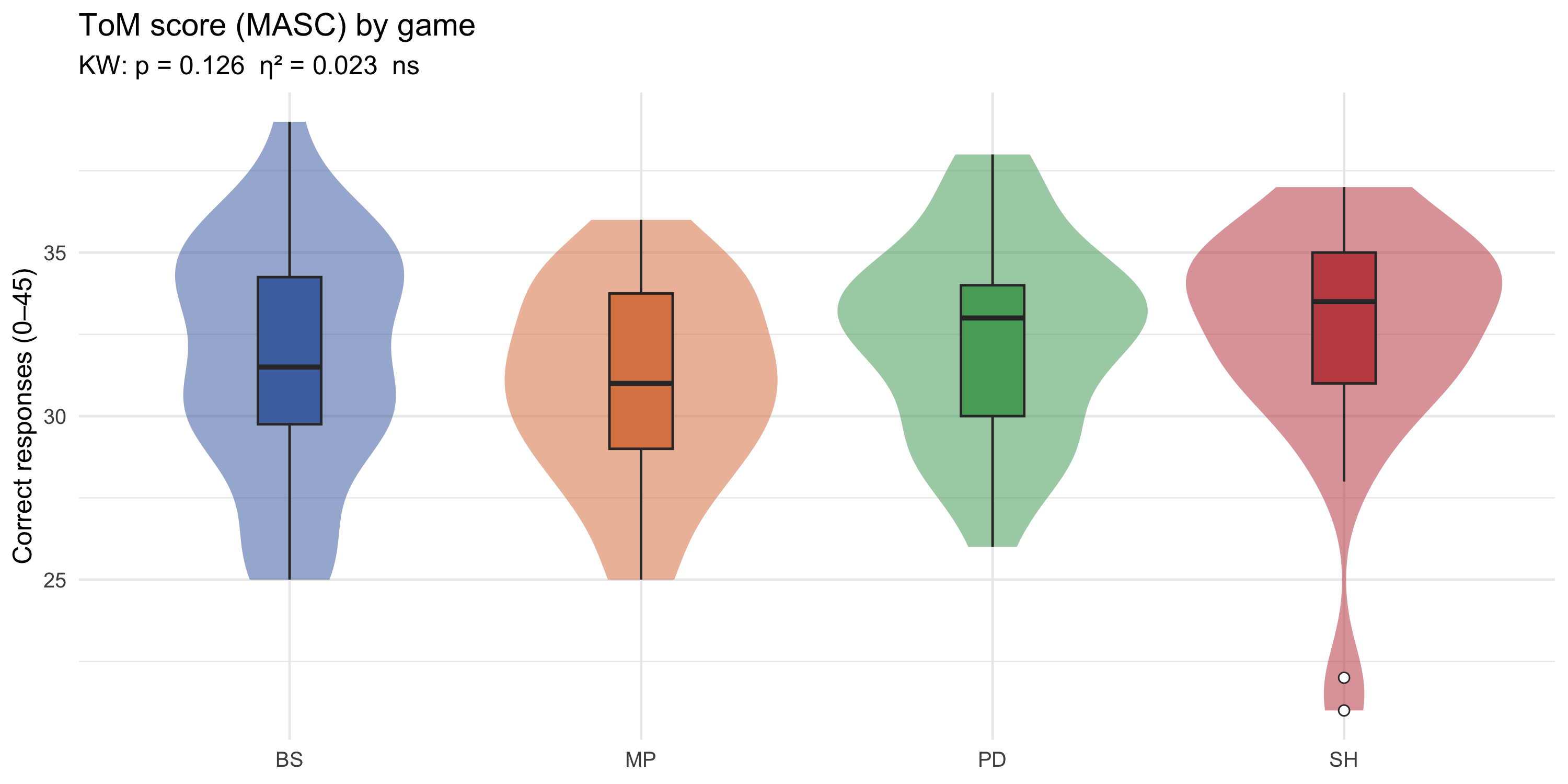
### ToM score distribution by game
```{r}
#| label: fig-violin-tom
#| fig-cap: "Distribution of total correct ToM score (0–40) by experimental condition."
#| fig-height: 5
p_violin_tom
```
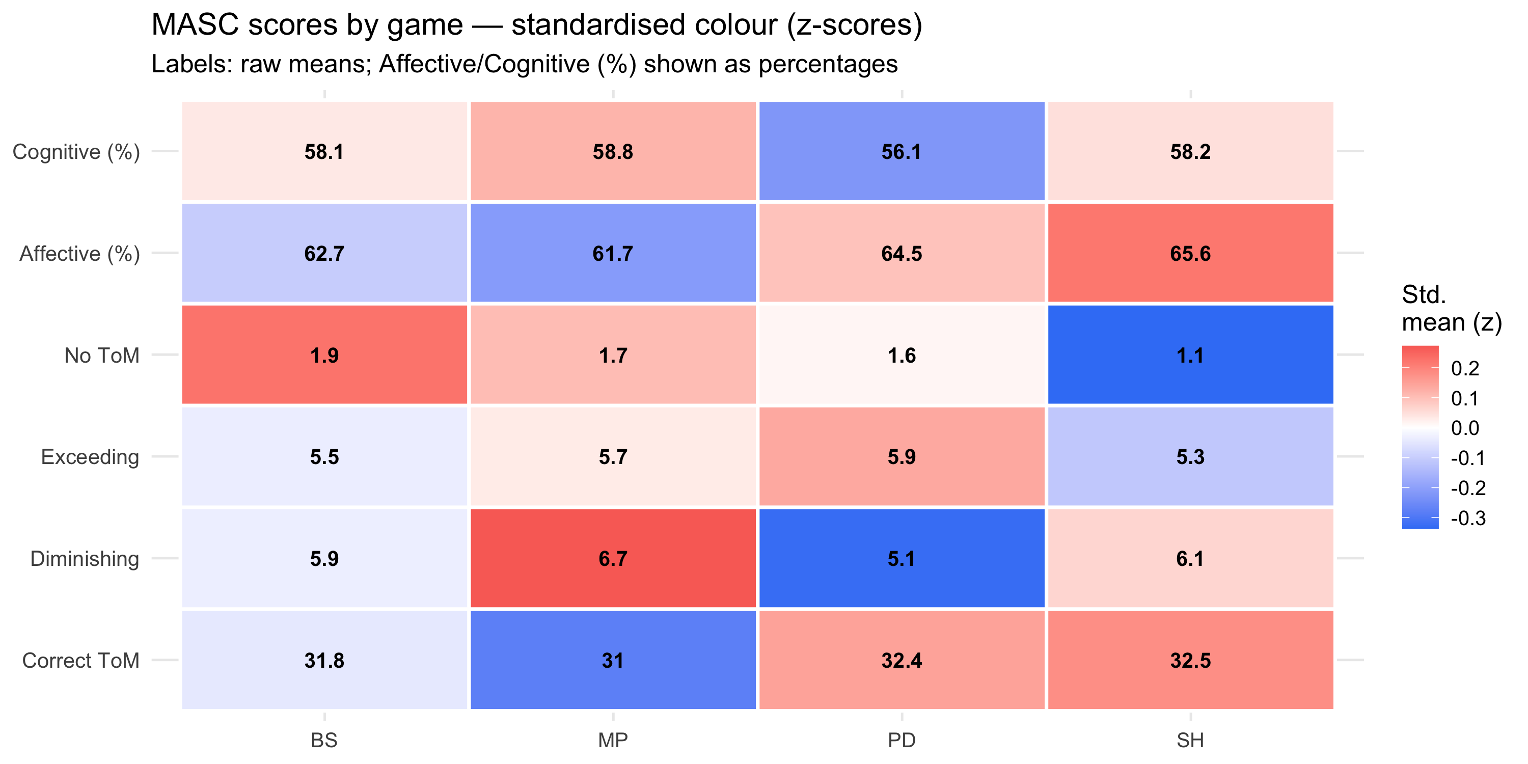
### MASC dimensions heatmap
```{r}
#| label: fig-heatmap
#| fig-cap: "Within-variable standardised means (z-scores) across games — colour encodes relative position within each dimension, making incompatible scales (0–40 count vs 0–1 proportion) comparable. Cell labels show raw means; Affective (%) and Cognitive (%) labels are multiplied ×100 for readability."
#| fig-height: 5
p_heat_masc
```
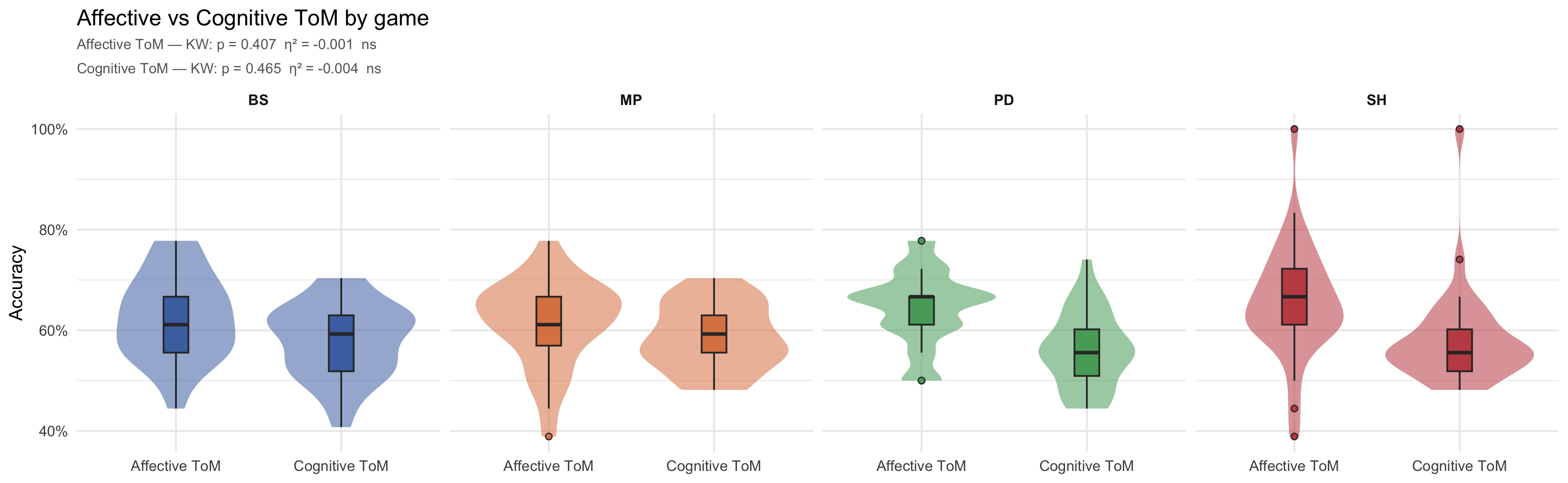
### Affective vs Cognitive ToM by game
```{r}
#| label: fig-aff-cog
#| fig-cap: "Distributions of affective and cognitive ToM accuracy by experimental condition. Accuracy displayed as proportion (0–1)."
#| fig-width: 13
#| fig-height: 4
p_aff_cog
```
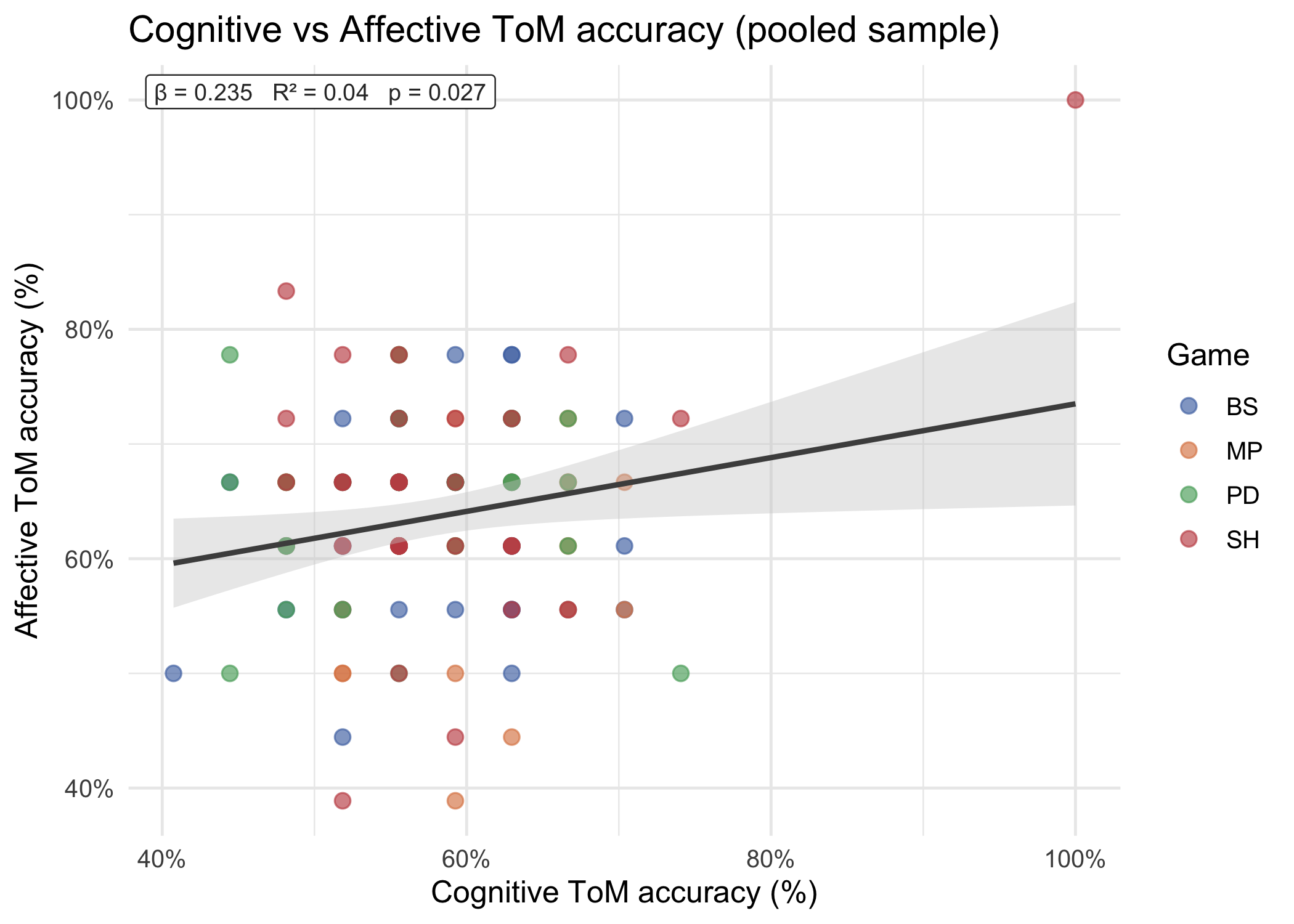
### Cognitive vs affective ToM scatter (pooled sample)
```{r}
#| label: fig-scatter
#| fig-cap: "Pooled scatter of cognitive vs affective ToM accuracy with a single OLS regression line (grey). The top-left label reports the slope (β), variance explained (R²), and significance of the linear fit. Points are coloured by game."
#| fig-width: 7
#| fig-height: 5
p_scatter
```
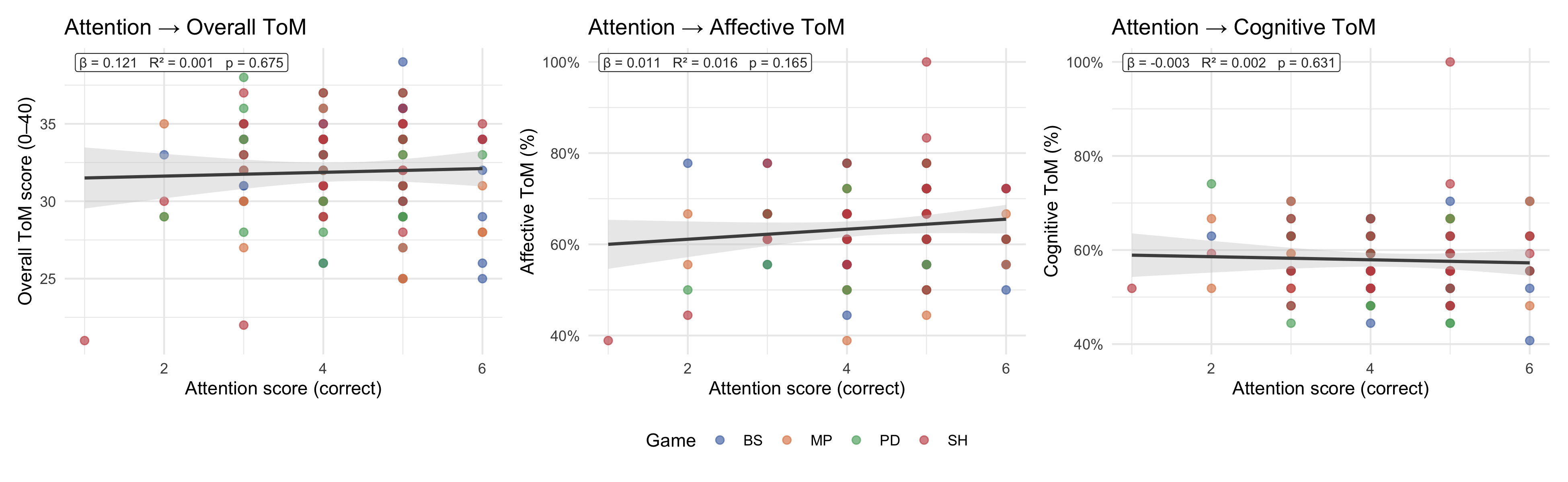
### Attention control vs ToM scores
The MASC includes attention-check items that do not require mental-state inference. Correlating the attention score with ToM scores helps assess whether performance differences are driven by general task engagement / comprehension rather than ToM ability per se.
```{r}
#| label: fig-attention
#| fig-cap: "Scatter plots of the MASC attention-check score against overall ToM score (left), affective ToM accuracy (centre), and cognitive ToM accuracy (right). Each panel shows an OLS line (grey band = 95% CI) and a top-left label reporting β, R², and p-value. Points are coloured by game."
#| fig-width: 13
#| fig-height: 4
p_attention_panel
```
::: callout-note
A strong positive association between attention score and ToM scores would indicate that overall task engagement (rather than ToM specifically) drives performance. A weak or absent association is more consistent with ToM scores reflecting the construct of interest.
:::
## IRI — Interpersonal Reactivity Index
### Descriptive statistics by game
```{r}
#| label: tab-iri
tab_iri
```
::: callout-note
Statistics are median (Q1, Q3). Kruskal-Wallis tests between games; η² effect sizes reported. Random assignment should yield comparable IRI profiles across conditions — any significant differences are relevant as potential confounders in subsequent analyses.
:::
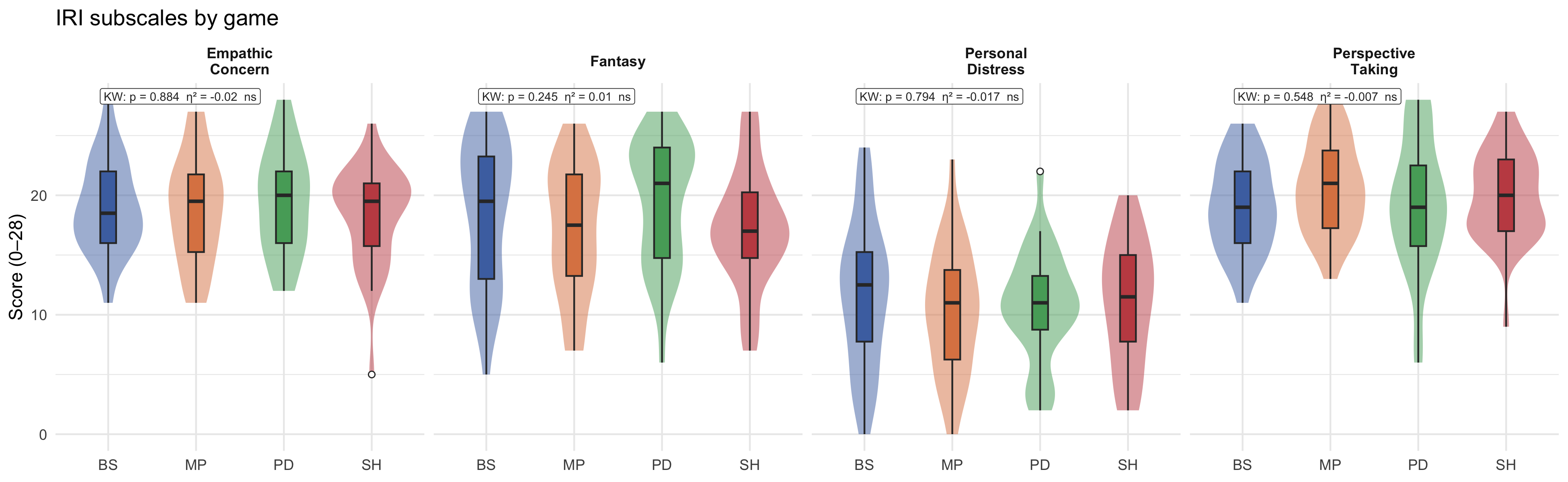
### IRI subscale distributions
```{r}
#| label: fig-iri-violin
#| fig-cap: "Distribution of the four IRI subscales across experimental conditions. Scores range from 0 to 28 per subscale."
#| fig-width: 13
#| fig-height: 4
p_iri_violin
```
### Internal consistency
Cronbach's α for the four-subscale block:
```{r}
#| label: iri-alpha
# psych::alpha() computed in code.R
print(iri_alpha, digits = 3)
```
::: callout-note
Note that Cronbach's α across the four IRI subscales reflects the internal consistency of the *battery as a whole* (treating the four subscales as items). High α indicates overlap between subscales; low α is expected and appropriate when the subscales capture distinct facets of empathy (the IRI was designed as a multi-dimensional instrument). Per-subscale reliability would typically be assessed at the item level.
:::
## MASC × IRI: correlations and regressions
```{r}
#| include: false
n_mi <- nrow(df_mi)
```
This section tests whether self-reported empathy (IRI) is associated with film-based ToM performance (MASC). Two complementary analyses are reported: targeted Spearman correlations to check whether *matching* pairs (affective ToM ↔ affective empathy; cognitive ToM ↔ cognitive empathy) are stronger than *crossing* ones, followed by binomial GLMs predicting MASC accuracy from the four IRI subscales simultaneously.
### Level A — Spearman correlations
```{r}
#| label: tab-spearman
tab_spearman |>
  gt() |>
  cols_label(
    MASC_dim = "MASC dimension",
    Pair     = "Pair",
    rho      = "\u03c1",
    p_fmt    = "p",
    sig      = "Sig."
  ) |>
  tab_header(
    title    = "Spearman correlations: MASC \u00d7 IRI",
    subtitle = paste0("N = ", n_mi,
                      " complete cases. Exact = FALSE (ties present).")
  ) |>
  tab_style(style = cell_text(weight = "bold"),
            locations = cells_column_labels()) |>
  tab_style(style = cell_text(weight = "bold"),
            locations = cells_body(columns = sig, rows = sig != "ns")) |>
  tab_footnote("* p < .05  ** p < .01  *** p < .001  ns = not significant")
```
::: callout-note
**Matching vs crossing hypothesis.** Affective ToM (emotion inference from film clips) is theorised to align more strongly with affective empathy (Empathic Concern, Personal Distress). Cognitive ToM (belief/intention inference) should align more with cognitive empathy (Perspective Taking). Pairs that cross the affective/cognitive boundary serve as a discriminant validity check — weaker or non-significant ρ there supports construct differentiation.
:::
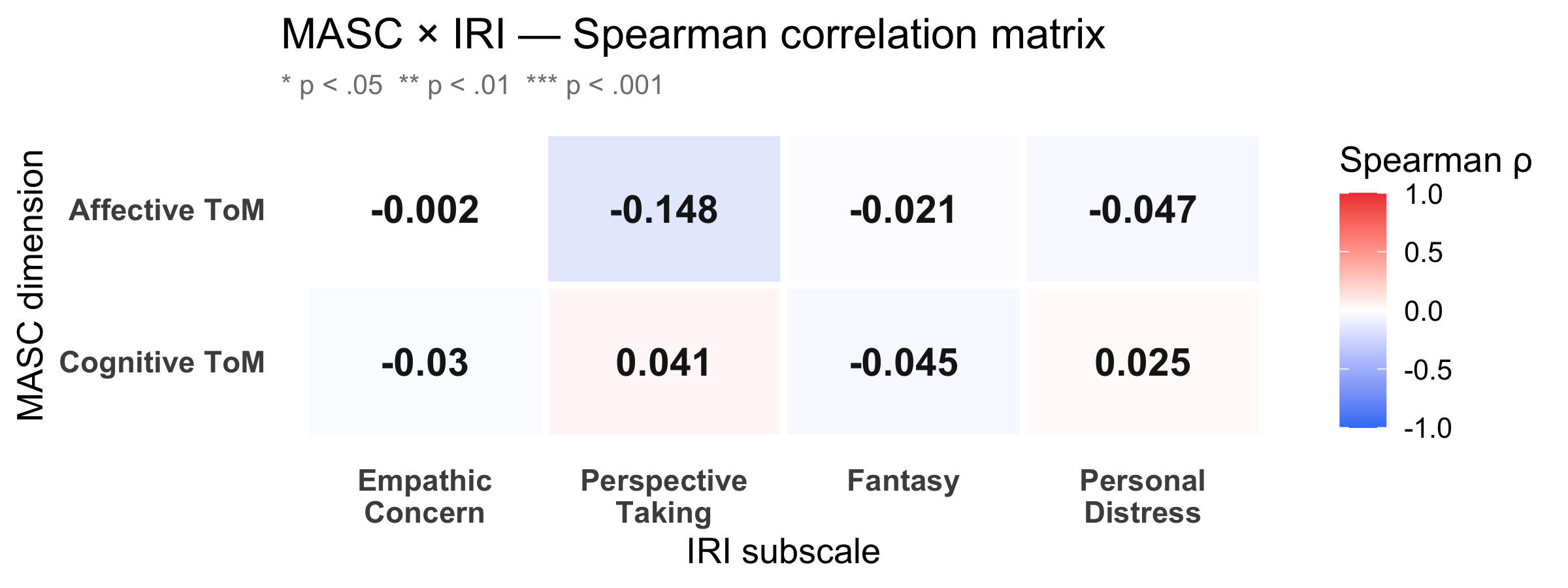
### Correlation heatmap
```{r}
#| label: fig-cor-heat
#| fig-cap: "Spearman ρ between the two MASC dimensions (rows) and the four IRI subscales (columns). Red = positive association, blue = negative. Significance stars: * p < .05 ** p < .01 *** p < .001."
#| fig-width: 8
#| fig-height: 3
p_cor_heat
```
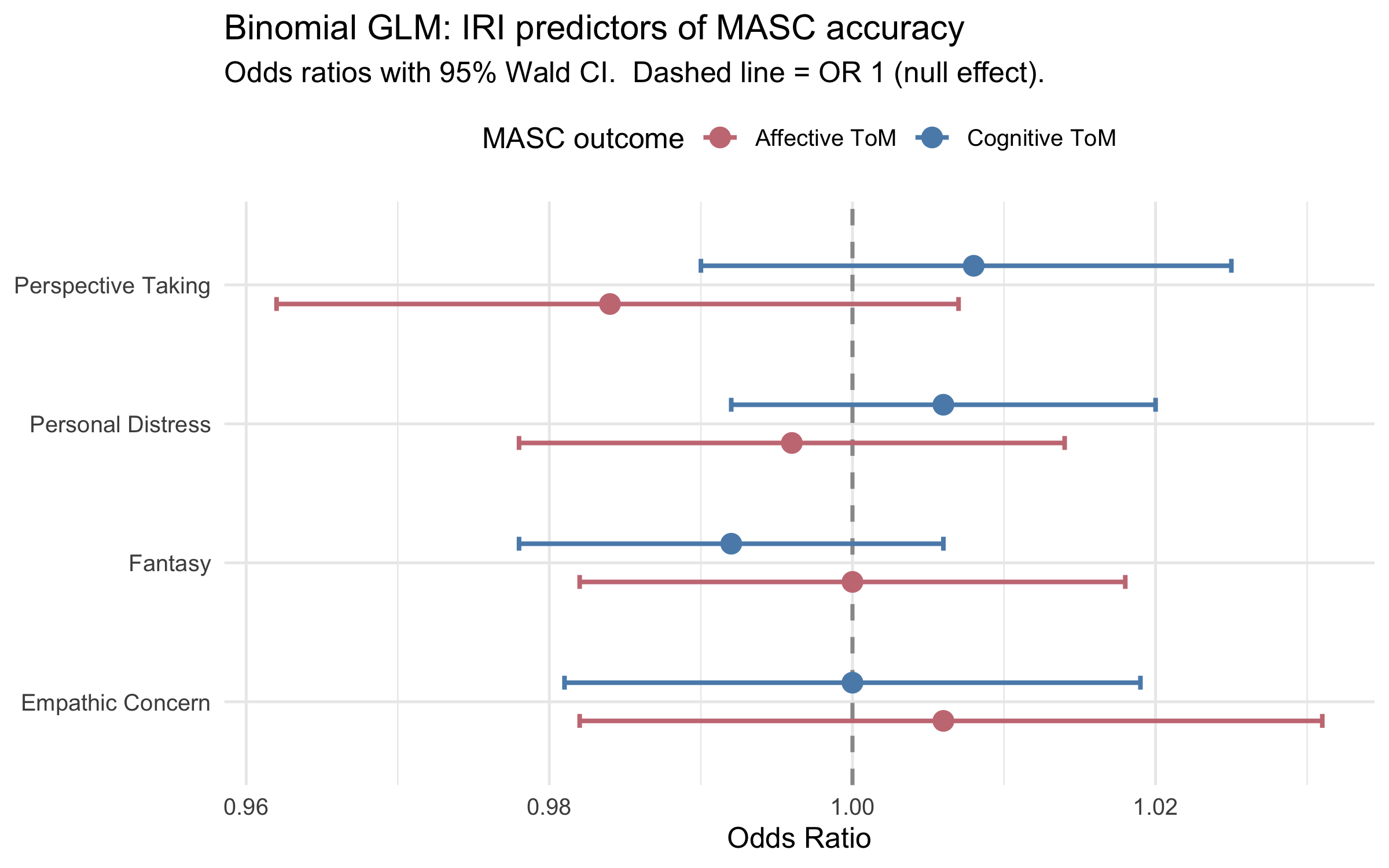
### Level B — Binomial GLMs
IRI subscales entered simultaneously as predictors of MASC accuracy. The response is modelled as a binomial count of correct answers (17 affective items; 28 cognitive items, total = 45). Coefficients are on the log-odds scale; the forest plot shows exponentiated odds ratios (OR) with 95% Wald CIs.
```{r}
#| label: tab-glm
tab_glm |>
  select(Outcome, Predictor, beta, SE, OR, OR_lo, OR_hi, stat, p_fmt, sig) |>
  gt() |>
  tab_header(
    title    = "Binomial GLM: IRI subscales predicting MASC accuracy",
    subtitle = "Family: binomial (logit link). Wald 95% CI."
  ) |>
  cols_label(beta = "\u03b2", SE = "SE", OR = "OR",
             OR_lo = "95% CI lo", OR_hi = "95% CI hi",
             stat = "z", p_fmt = "p", sig = "Sig.") |>
  tab_row_group(label = "Outcome: Cognitive ToM (28 items)",
                rows = Outcome == "Cognitive ToM") |>
  tab_row_group(label = "Outcome: Affective ToM (17 items)",
                rows = Outcome == "Affective ToM") |>
  tab_style(style = cell_text(weight = "bold"),
            locations = cells_column_labels()) |>
  tab_style(style = cell_text(weight = "bold"),
            locations = cells_body(columns = sig, rows = sig != "")) |>
  tab_style(style = cell_text(weight = "bold", color = "#2d7a3a"),
            locations = cells_row_groups()) |>
  tab_footnote("\u03b2 = log-odds coefficient. OR = exp(\u03b2). Wald 95% CI. * p < .05  ** p < .01  *** p < .001.")
```
::: callout-note
**Overdispersion check.** A binomial GLM assumes variance = μ(1−μ)/n; real data often show extra-binomial variation (overdispersion). The dispersion parameter φ is estimated by the quasi-binomial fit: **φ(affective) = `r disp_aff`**, **φ(cognitive) = `r disp_cog`**. φ ≈ 1 means the binomial assumption holds; φ >> 1 means SEs from the standard binomial are underestimated. The quasi-binomial robustness check below quantifies the difference.
:::
```{r}
#| label: fig-glm-forest
#| fig-cap: "Forest plot: odds ratios from the binomial GLMs. Error bars = 95% Wald CI. Dashed line = OR 1 (null effect)."
#| fig-width: 8
#| fig-height: 5
p_glm_forest
```
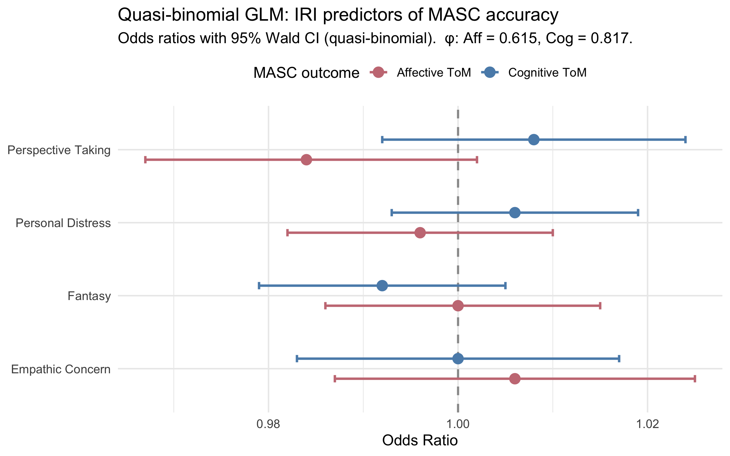
### Quasi-binomial robustness check
The quasi-binomial model uses the same formula but estimates a free dispersion parameter φ, inflating standard errors by √φ. Coefficients (β) and odds ratios are **identical** to the binomial — only SEs and p-values change. The comparison table shows directly where overdispersion changes inference.
```{r}
#| label: tab-glm-compare
tab_glm_compare |>
  select(Outcome, Predictor, beta, OR,
         SE_binom, SE_quasi, SE_ratio,
         p_binom, sig_binom, p_quasi, sig_quasi) |>
  gt() |>
  tab_header(
    title    = "Binomial vs quasi-binomial: SE and p-value comparison",
    subtitle = paste0("φ (dispersion): Affective = ", disp_aff,
                      ", Cognitive = ", disp_cog,
                      ". SE ratio \u2248 \u221a\u03c6.")
  ) |>
  cols_label(
    beta      = "\u03b2", OR = "OR",
    SE_binom  = "SE (binom)", SE_quasi = "SE (quasi)", SE_ratio = "SE ratio",
    p_binom   = "p (binom)",  sig_binom = "Sig. (binom)",
    p_quasi   = "p (quasi)",  sig_quasi = "Sig. (quasi)"
  ) |>
  tab_row_group(label = "Outcome: Cognitive ToM",
                rows = Outcome == "Cognitive ToM") |>
  tab_row_group(label = "Outcome: Affective ToM",
                rows = Outcome == "Affective ToM") |>
  tab_style(style = cell_text(weight = "bold"),
            locations = cells_column_labels()) |>
  tab_style(style = cell_text(weight = "bold", color = "#2d7a3a"),
            locations = cells_row_groups()) |>
  tab_style(
    style = cell_fill(color = "#fff3cd"),
    locations = cells_body(
      columns = c(sig_binom, sig_quasi),
      rows = sig_binom != sig_quasi
    )
  ) |>
  tab_footnote("Yellow highlight = significance changes between models. SE ratio = SE\u2098\u1d64\u1d43\u02e2\u1d35 / SE\u1d47\u1d35\u207f\u1d52\u1d50.")
```
```{r}
#| label: fig-glm-forest-quasi
#| fig-cap: "Forest plot: odds ratios from the quasi-binomial GLMs. Wider CIs reflect SE inflation by √φ. Compare with the binomial forest plot above."
#| fig-width: 8
#| fig-height: 5
p_glm_forest_quasi
```
## Conditioning on gender and role
The preceding analyses compare MASC and IRI scores across experimental games without accounting for sample composition. Since participants were not stratified by demographics at assignment, observed game-level differences in ToM and empathy scores may be confounded by gender composition or by the structural difference between experimental sites (P1 = LEEN laboratory; P2 = CoCoLab). This section (i) visualises distributions stratified by gender and role, and (ii) fits OLS models with game, gender, and role entered simultaneously as predictors. The reference category for all models is: game = BS, gender = Male, role = P1 (LEEN).
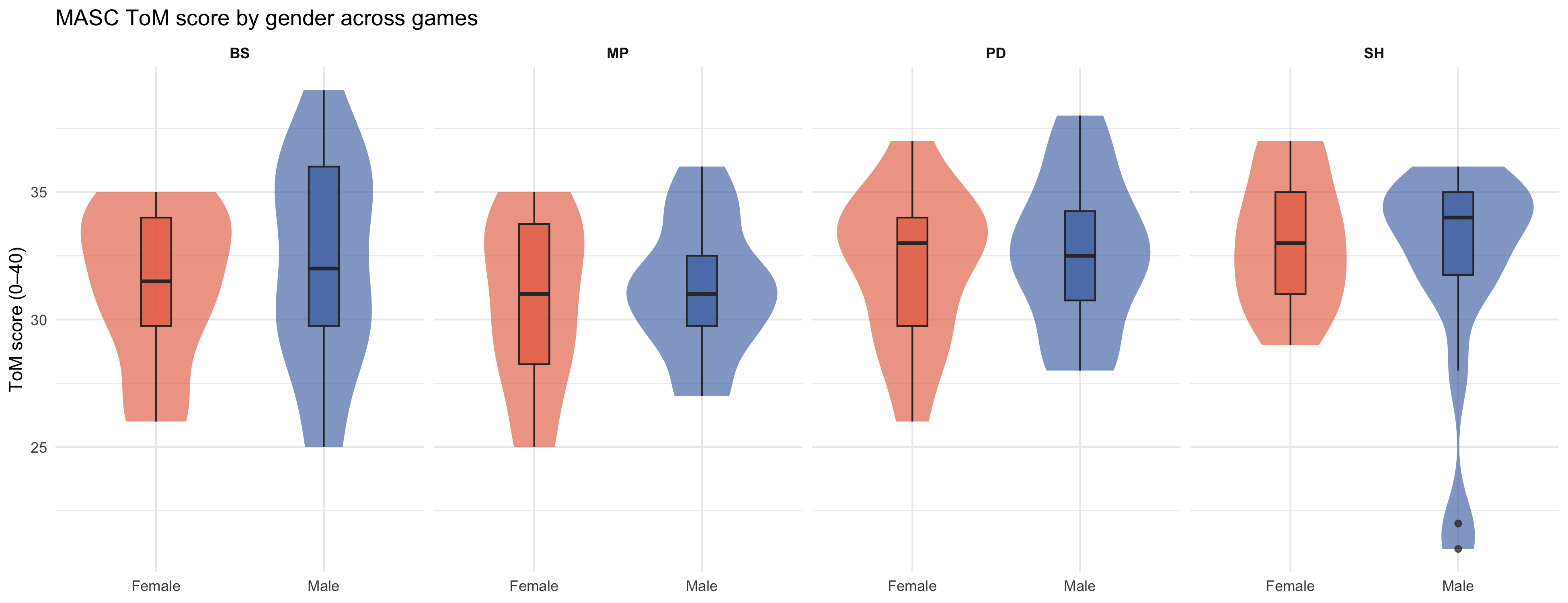
### MASC by gender
```{r}
#| label: fig-masc-gender
#| fig-cap: "MASC overall ToM score by gender within each game condition. Violin + box plot; no legend (Male = blue, Female = orange)."
#| fig-width: 13
#| fig-height: 5
p_masc_gender
```
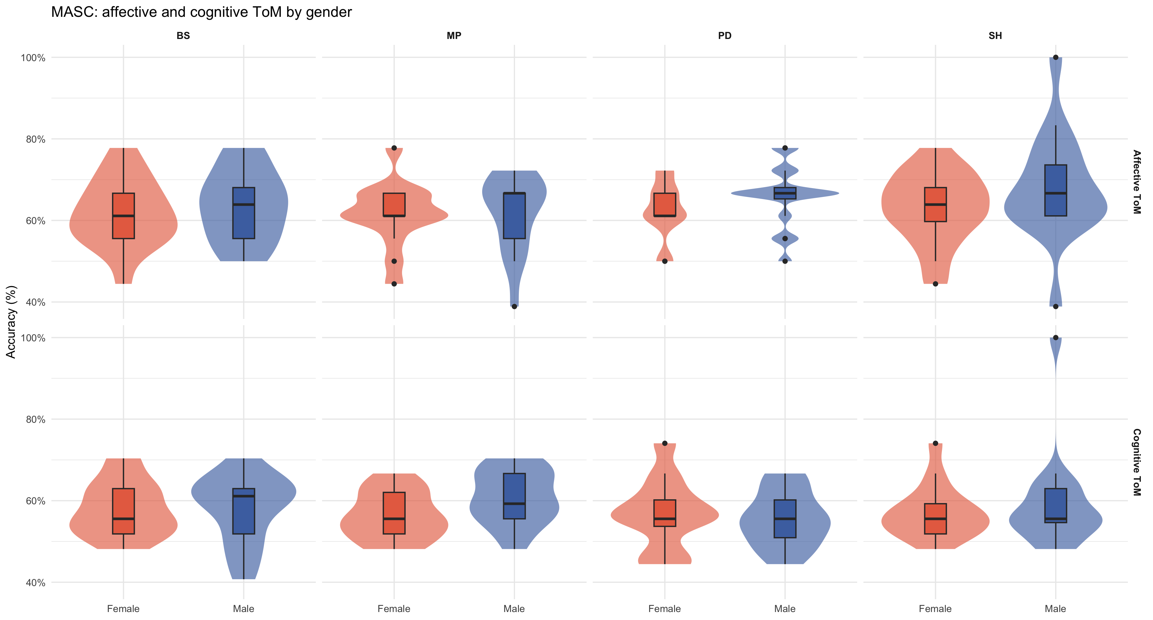
```{r}
#| label: fig-masc-dim-gender
#| fig-cap: "MASC affective and cognitive ToM accuracy by gender, faceted by game (columns) and dimension (rows)."
#| fig-width: 13
#| fig-height: 7
p_masc_dim_gender
```
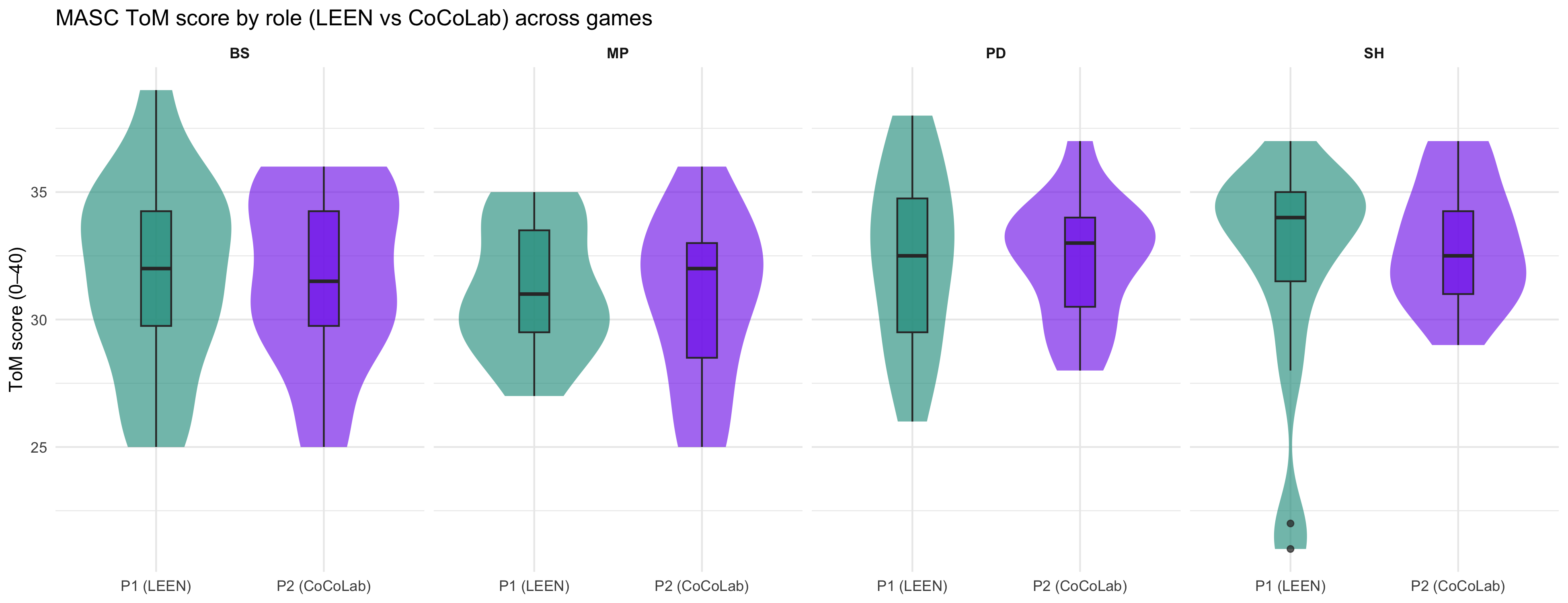
### MASC by role
```{r}
#| label: fig-masc-role
#| fig-cap: "MASC overall ToM score by experimental role (P1 LEEN vs P2 CoCoLab) within each game. Violin + box plot."
#| fig-width: 13
#| fig-height: 5
p_masc_role
```
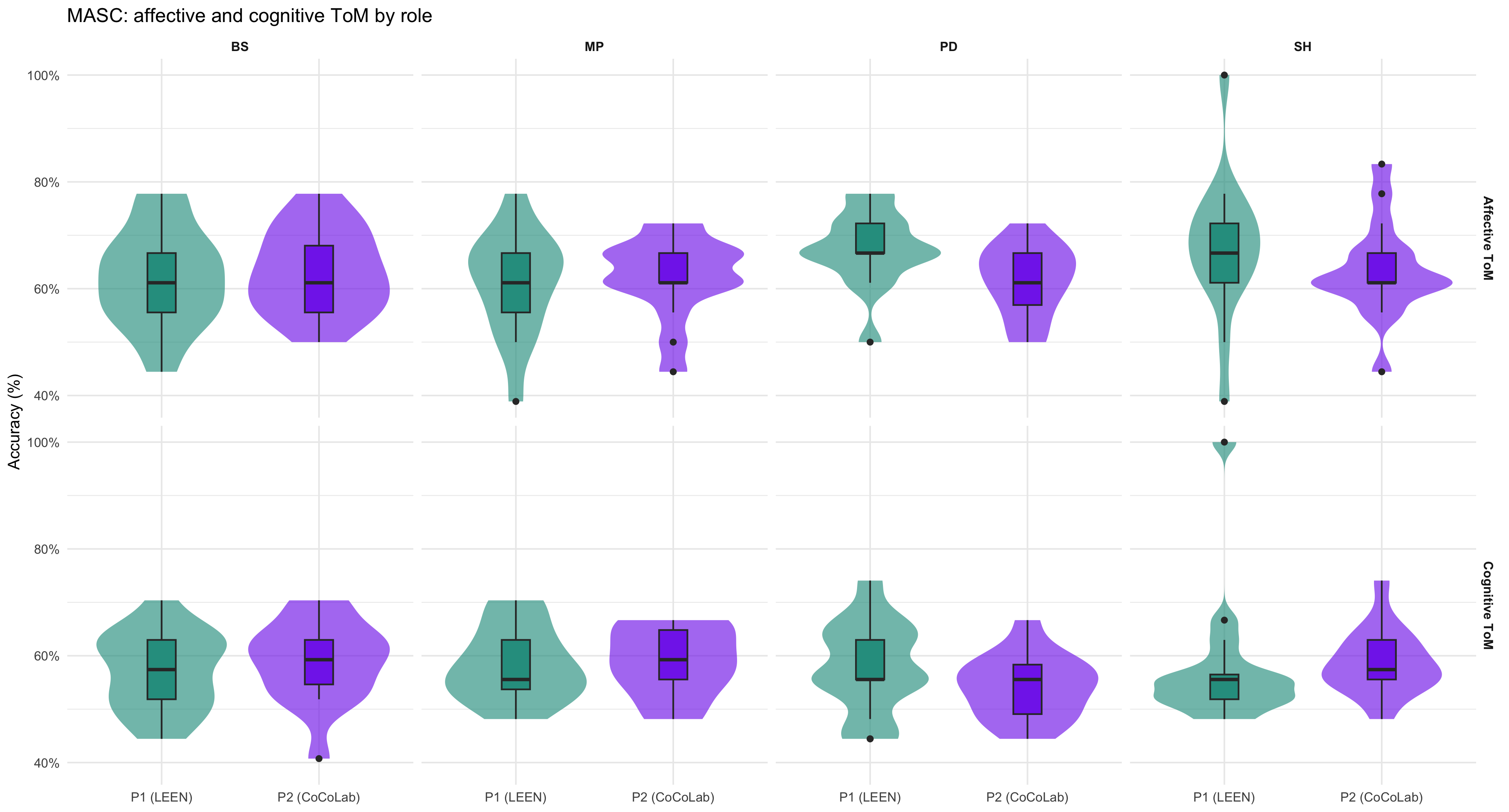
```{r}
#| label: fig-masc-dim-role
#| fig-cap: "MASC affective and cognitive ToM accuracy by role, faceted by game (columns) and dimension (rows)."
#| fig-width: 13
#| fig-height: 7
p_masc_dim_role
```
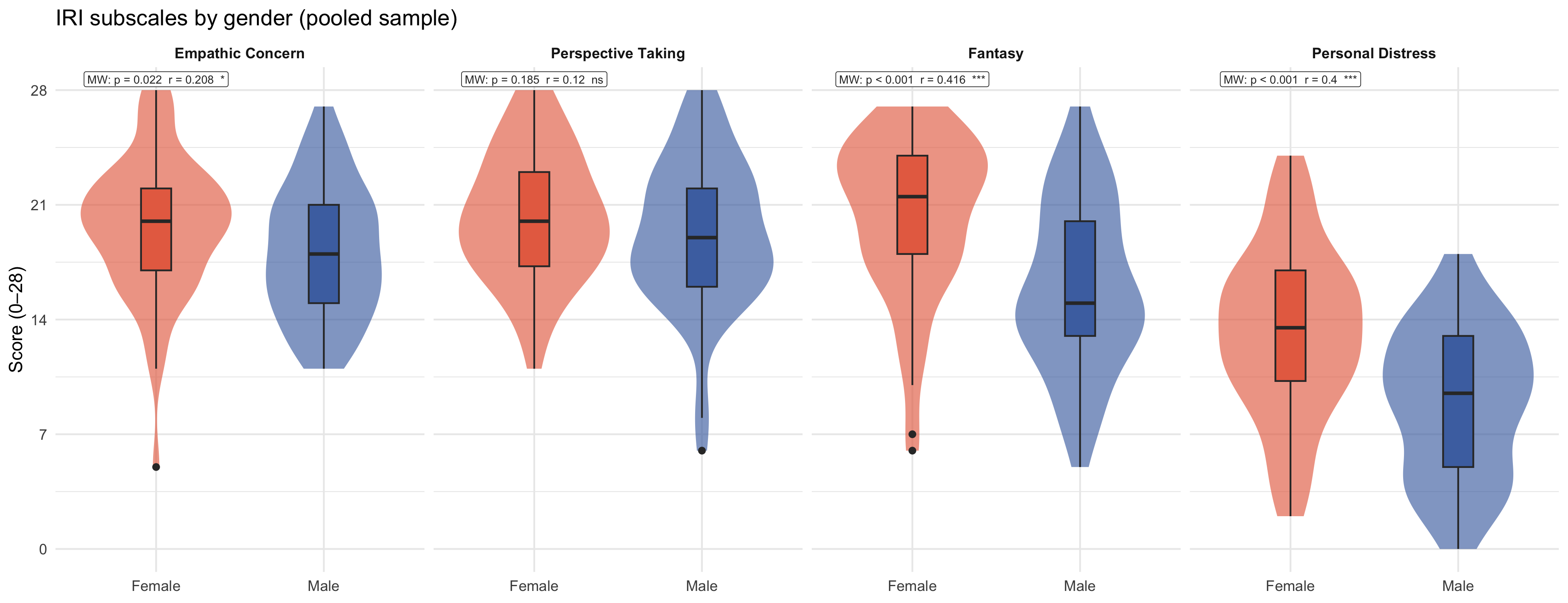
### IRI by gender
```{r}
#| label: fig-iri-gender
#| fig-cap: "IRI four subscales by gender (pooled sample). All subscales on the same y-axis (0–28) for comparability."
#| fig-width: 13
#| fig-height: 5
p_iri_gender
```
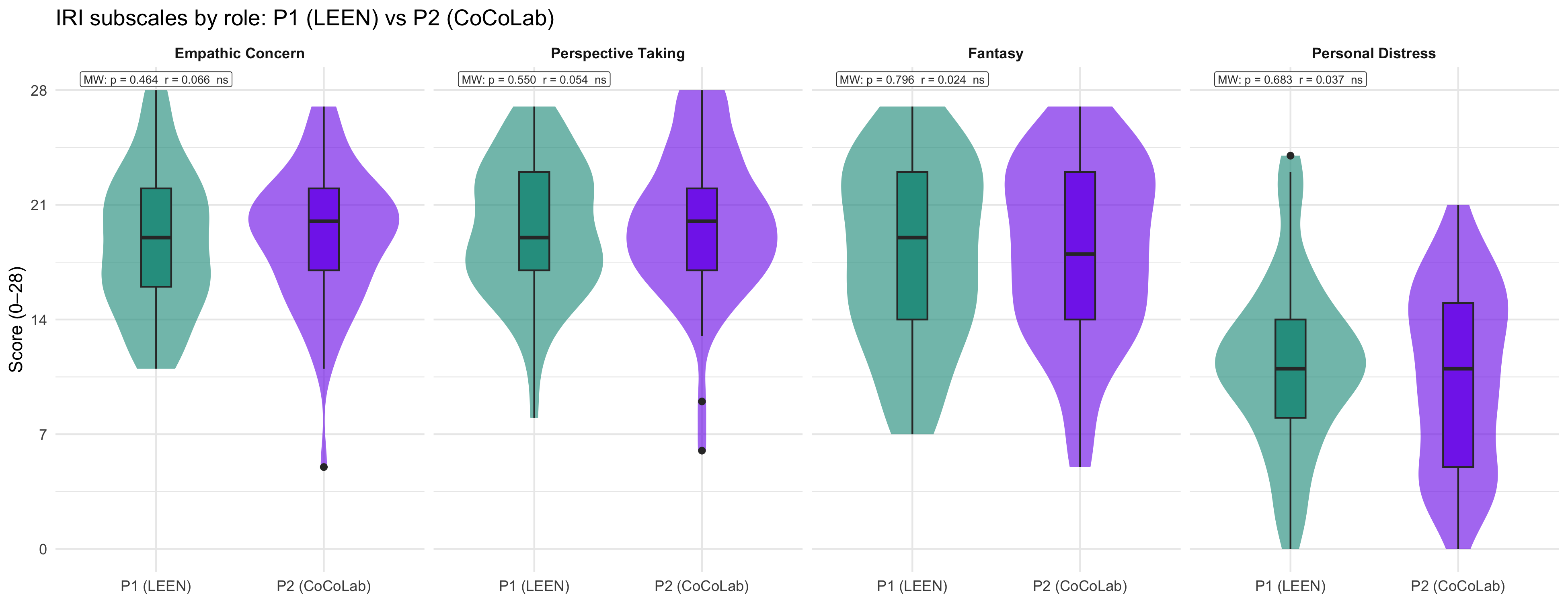
### IRI by role
```{r}
#| label: fig-iri-role
#| fig-cap: "IRI four subscales by experimental role: P1 (LEEN) vs P2 (CoCoLab), pooled across games."
#| fig-width: 13
#| fig-height: 5
p_iri_role
```
### OLS regressions with demographic controls
**MASC models** — outcome variables are overall ToM score (0–40) and the two proportion scores (affective, cognitive), each regressed on game condition, gender, and role simultaneously.
```{r}
#| label: tab-ols-masc
gt_ols_masc
```
```{r}
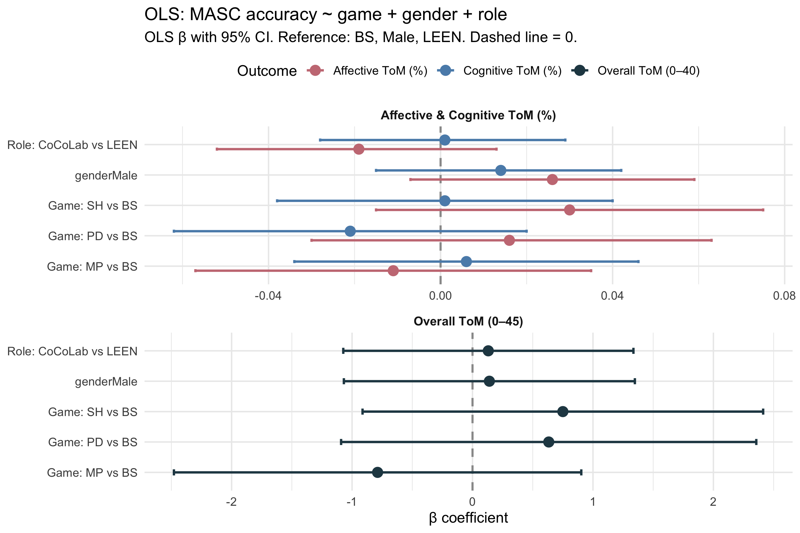
#| label: fig-forest-masc8
#| fig-cap: "Forest plot: OLS β coefficients with 95% CI for MASC outcomes. Dashed line = 0 (null effect). All three outcomes shown simultaneously; note that scales differ (0–40 vs proportion)."
#| fig-width: 9
#| fig-height: 6
p_forest_masc8
```
**IRI models** — each of the four subscales (0–28) regressed on game, gender, and role.
```{r}
#| label: tab-ols-iri
gt_ols_iri
```
```{r}
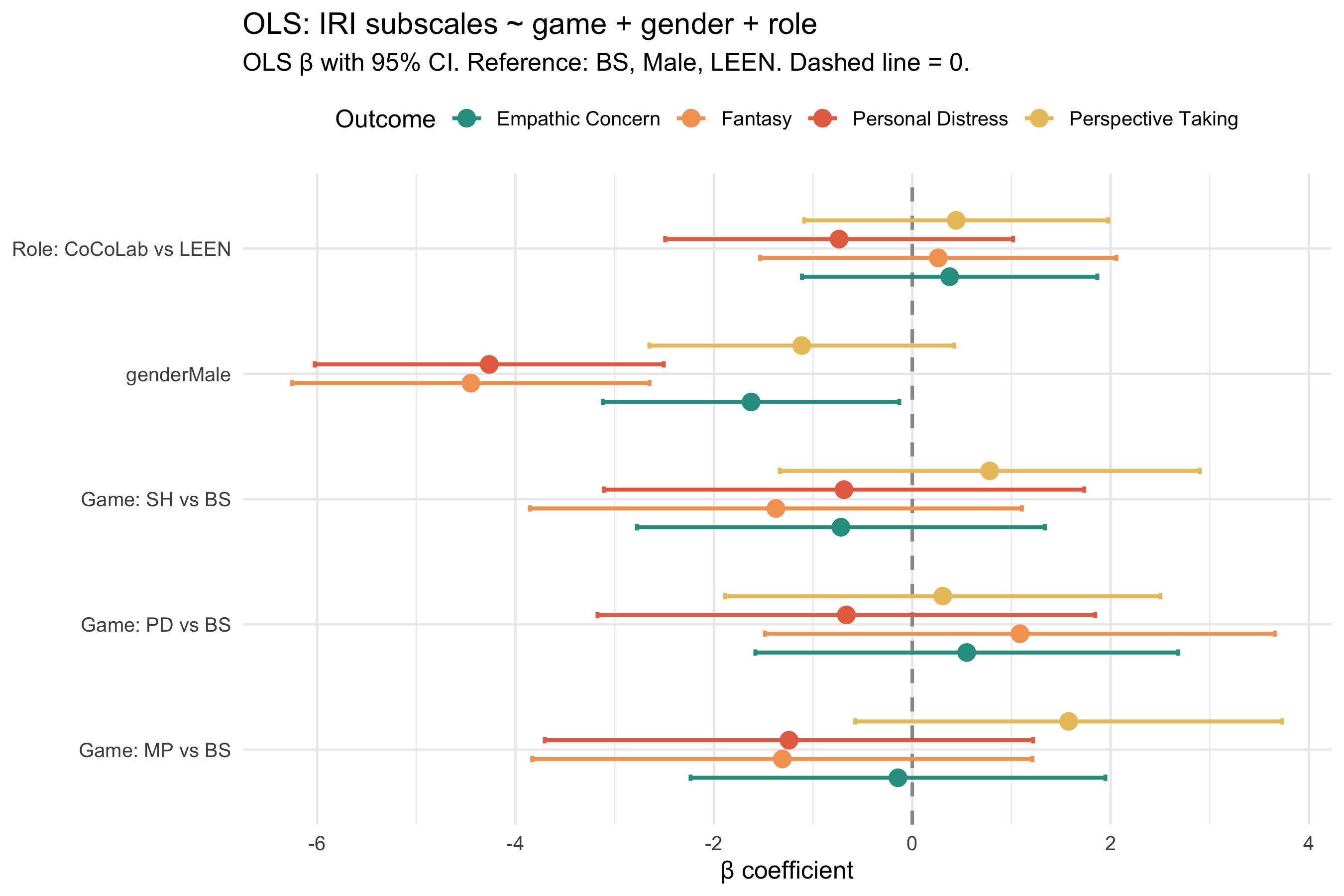
#| label: fig-forest-iri8
#| fig-cap: "Forest plot: OLS β coefficients with 95% CI for IRI subscales. Game effects (vs BS), gender effect (Female vs Male), and role effect (CoCoLab vs LEEN) shown side by side."
#| fig-width: 9
#| fig-height: 6
p_forest_iri8
```
::: callout-note
**Interpretation note.** Game coefficients in these models represent the *conditional* effect of game assignment given equal gender and role composition. A game coefficient that is significant unconditionally (Kruskal-Wallis in sections 4–5) but non-significant here suggests partial confounding by demographics. Conversely, a gender or role coefficient reveals systematic differences in MASC/IRI scores attributable to those characteristics independently of game.
:::
## Response times & processing speed
Cognitive and affective tasks vary in the time required for deliberation and response. This section examines whether **speed of processing** correlates with **accuracy** across the MASC (ToM), IRI (empathy), and CRT (reflection), and whether games differ in time investment.
### MASC response times by dimension
```{r}
#| label: tab-resp-times
tab_resp_times
```
### MASC: speed–accuracy trade-off
```{r}
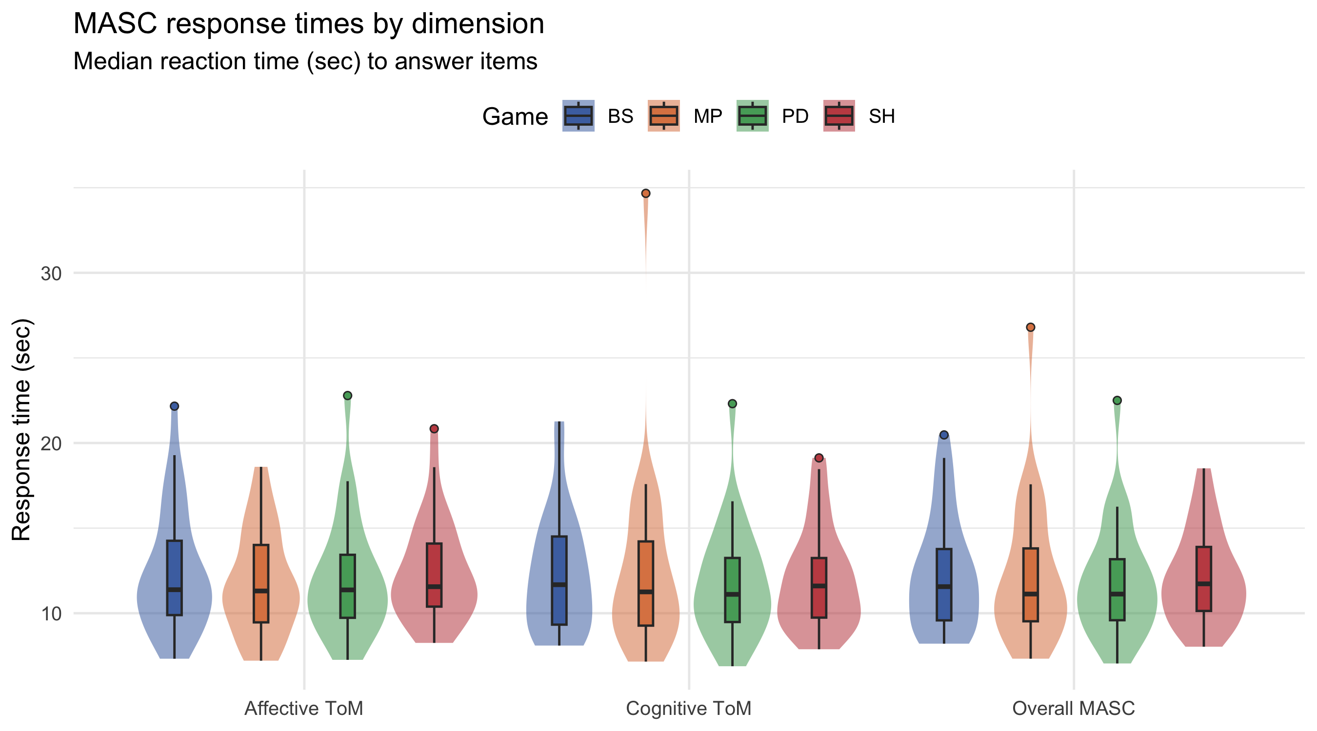
#| label: fig-masc-rt-violin
#| fig-cap: "Distribution of MASC response times by dimension (overall / affective / cognitive) across games. Violin width = density; box plot = quartiles. Faster response times may reflect overconfidence or heuristic use; slower times suggest deliberative mentalising."
#| fig-width: 9
#| fig-height: 5
p_masc_rt
```
```{r}
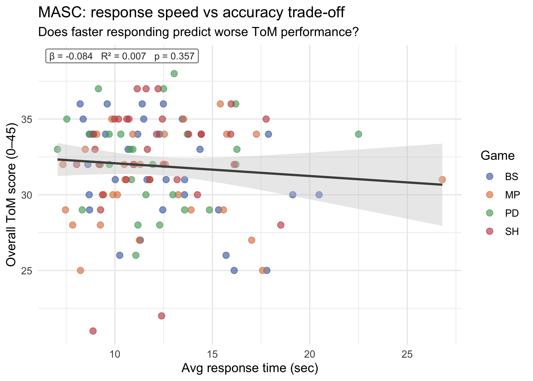
#| label: fig-masc-speed-accuracy
#| fig-cap: "MASC: average response time vs overall ToM accuracy. Does faster responding predict worse accuracy (speed–accuracy trade-off)? OLS line fitted on pooled sample; top-left label reports β, R², p-value."
#| fig-width: 7
#| fig-height: 5
p_masc_speed_accuracy
```
::: callout-note
**Speed–accuracy trade-off in ToM.** If participants who respond faster are less accurate, this suggests a speed–accuracy trade-off: quick responses may rely on superficial heuristics rather than genuine mentalising. Conversely, a positive correlation (faster = more accurate) would indicate fluent, confident mentalising. A near-zero correlation indicates speed and accuracy are independent — both may reflect trait differences in responding style (e.g. impulsivity) rather than true mentalising ability.
:::
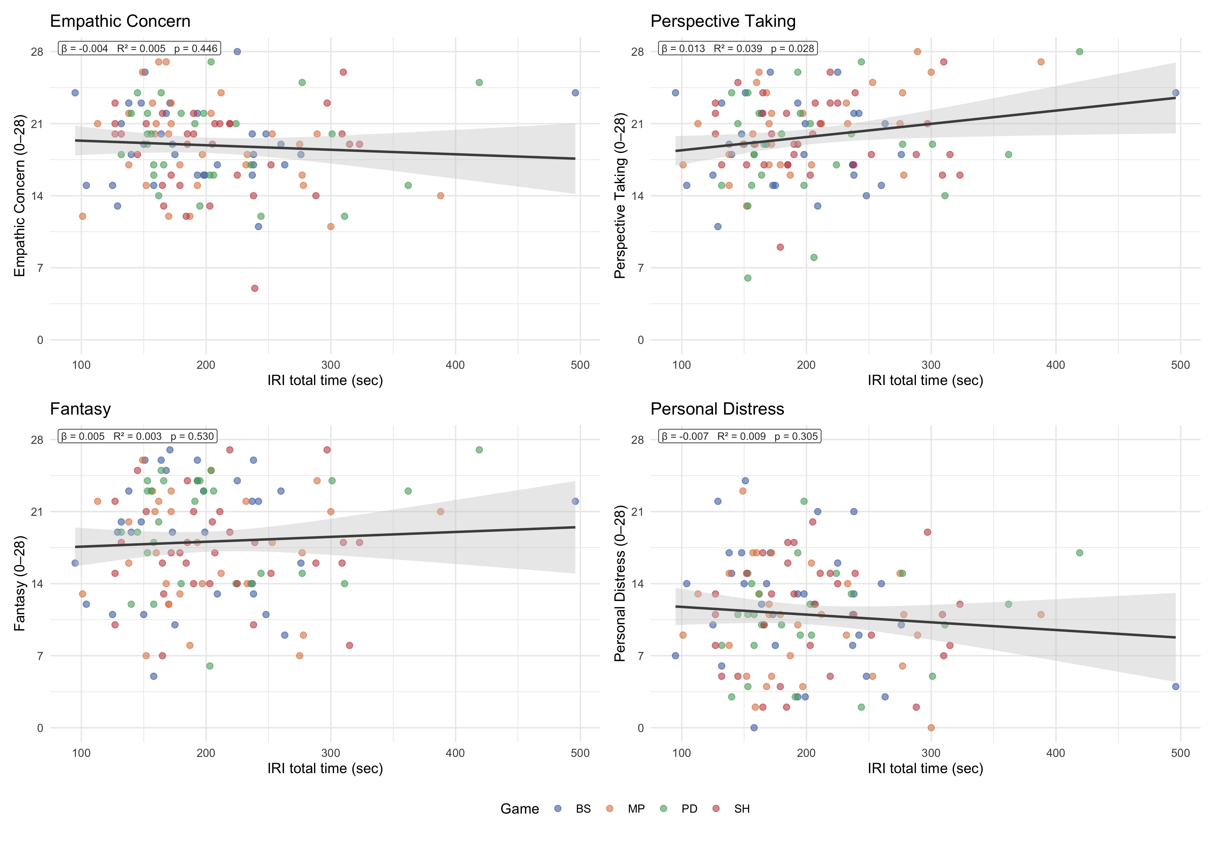
### IRI: time spent vs all subscales
```{r}
#| label: fig-iri-speed-panel
#| fig-cap: "IRI total completion time vs each of the four subscales (Empathic Concern, Perspective Taking, Fantasy, Personal Distress). Each panel shows an OLS line with 95% CI and a top-left annotation reporting β, R², and p-value. All subscales share the same y-axis scale (0–28). Points coloured by game condition."
#| fig-width: 13
#| fig-height: 9
p_iri_speed_panel
```
## Preliminary interpretation
```{r}
#| echo: false
med_tom <- round(median(df$MASC_ToM_score, na.rm = TRUE), 1)
iqr_tom <- round(IQR(df$MASC_ToM_score, na.rm = TRUE), 1)
med_aff <- round(median(df$MASC_affective_perc_score, na.rm = TRUE), 3)
med_cog <- round(median(df$MASC_cognitive_perc_score, na.rm = TRUE), 3)
wil_p <- signif(wilcox_res$p.value, 2)
wil_es <- round(wilcox_es$effsize, 2)
wil_mag <- as.character(wilcox_es$magnitude)
```
The sample shows a median MASC ToM score of **`r med_tom`** (IQR = `r iqr_tom`) out of 40 items, consistent with adequate mentalising ability in a non-clinical adult population. The affective component (median `r med_aff*100`%) and the cognitive component (median `r med_cog*100`%) are compared within individuals: the Wilcoxon signed-rank test yields p = `r wil_p`, with a `r wil_mag` effect size (r = `r wil_es`), suggesting `r if(wil_p < 0.05) "a statistically significant" else "no significant"` difference between the two ToM dimensions at the sample level.
The attention-scatter plots provide a first check on whether task engagement confounds ToM performance — interpretation depends on the slope and confidence interval of the regression lines.
Differences in MASC profiles across games are informative to the extent that randomisation was imperfect or that participant sorting occurred. Any significant Kruskal-Wallis effects will be noted as potential covariates in the inferential sections (Parts II–III).
For the IRI, randomly assigned groups should show comparable empathy profiles. Significant game differences would flag imbalance that warrants covariate adjustment in the main analyses.